Non-covalent interaction visualized

Non-covalent interactions like hydrogen bond, van der Waals interactions, steric clashes can be visualized using a tool called Non-Covalent Interaction Index (NCI) based on the charge density and it’s gradient ( 10.1021/ja100936w).

The reduced density gradient (RDG), is a dimensionless quantitiy calculated using the density and its derivative. It can be expressed as (for spin degenerate system):

\[\begin{aligned} s(\mathbf{r}) &= \frac{|\nabla \rho(\mathbf{r})|}{2 k_F \rho(\mathbf{r})}\\ &=\frac{1}{2\left(3 \pi^2\right)^{1 / 3}} \frac{|\nabla \rho(\mathbf{r})|}{\rho(\mathbf{r})^{4 / 3}} \end{aligned},\]

where $k_F$ is the Fermi vector. The RDG ($s(\mathbf{r})$) describes the degree of deviation of the charge density from homogeneous electron gas. For homogeneous electron gas, the RDG is always $0$.

For typical covalent interactions, the RDG are small due to the high concentration of electron denstiy. However, for regions with low density, only when the gradient is also small will the NCI be small. This can happen when there are some degrees of non-covalent interactions (can be attrative or repulsive to the electron) exist in the system. Using both the electron density and the RDG, one can easily identify regions where non-covalent interaction is taking place.

To calculate the RDG, we first need to calculate the gradient of the charge density. With VASP’s CHGCAR, we can use the central finite difference to obtain the gradient:

\[\nabla f(\vec r)=\left[\begin{array}{c} \frac{\partial f}{\partial a}(\vec r) \\ \frac{\partial f}{\partial b}(\vec r) \\ \frac{\partial f}{\partial c}(\vec r) \end{array}\right] \approx \frac{1}{2 h}\left[\begin{array}{c} [f\left(\vec r+e_a h_a\right)-f\left(\vec r-e_a h_a\right)]/(2h_a) \\ [f\left(\vec r+e_b h_b\right)-f\left(\vec r-e_b h_b\right)]/(2h_b) \\ [f\left(\vec r+e_c h_c\right)-f\left(\vec r-e_c h_c\right)]/(2h_c) \\ \end{array}\right],\]

where $a$, $b$ and $c$ index the lattice vectors and $h$ is the infinitestimal small values along the lattice vecotrs. We can easily obtain $\nabla f(\vec r)$ using the direct coordinates.

When the lattice vectors are not orthogonal to each other, according to the chain rule of partial derivation we have, for example the $x$-component of the $\nabla_c f(\vec r)$:

\[\frac{\partial}{\partial x} f(a,b,c) = \frac{\partial f}{\partial a} \frac{\partial a}{\partial x} + \frac{\partial f}{\partial b} \frac{\partial b}{\partial x} + \frac{\partial f}{\partial c} \frac{\partial c}{\partial x}\]

and similar for the $y$ and $z$ components. We can write $\nabla_c f(\vec r)$ in a more compact form as:

\[\nabla_c f(\vec r) = g \nabla f(\vec r)\]

where $g$ is a 3$\times$3 matrix with components corresponding to $\frac{\partial u}{\partial x}$ etc., and can be used to that transform the Cartesian coordinates to direct coordinates:

\[[x,y,z] g = [a,b,c]\]

Once we have obtained the gradient of the charge density at each point, we simply take the mod of it and follow Eq. 1 to calculate the RDG.

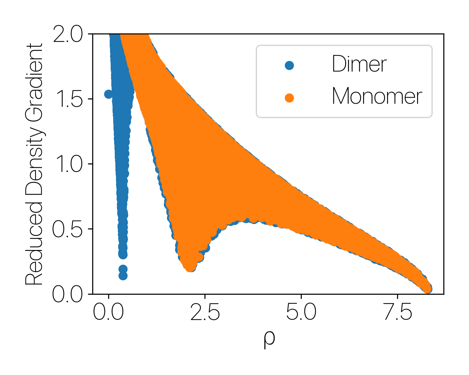
Using Water molecules as an example, by plotting the RDG vs $\rho$, we see that for a monomer (single water molecule), there’s no low density - low RDG poins, meaning that no non-covalent interacitve is found. The same plot for two water molecule shows a strong peak at low density, indicating that there’s a strong non-covalent interaction.

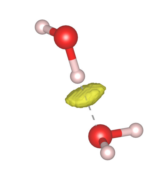
By plotting the these low $\rho$, low RDG points in real space, we see that they do exist between one water molecule’s H atom and the O atom of the other water molecule.

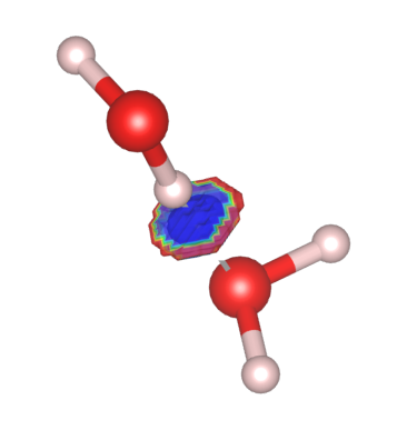
To identify the type of the non-covalent interaction (attractive or repulsive to the electrons), one can color the RDG isosurface using the eigenvalues of the Hessian of the denstiy (sometimes this is called the Non-Covalent Interaction Index). Sorting the eigenvalues of the Hessian, one finds that the sign of the middle eigenvalue determines the type of interaction. i.e. negative second eigenvalue of the Hessian corresponds to an attractive interaction to the electrons while a positive sign means the interaction is repulsive. Heuristicall (according to this post), one can color the isosurface of RDG with $\mathrm{sign}(\lambda_2)\rho(\vec r)$ where $\mathrm{sign}(\lambda_2)$ is the sign of the middle eigenvalue of the Hessian.

With VASP’s CHGCAR, we can perform similar central finite difference method to obtain the Hessian matrix element:

\[\frac{\partial^2 f}{\partial x_i \partial x_j} \approx \frac{f\left(x+e_i h+e_j h\right)-f\left(x+e_i h-e_j h\right)-f\left(x-e_i h+e_j h\right)+f\left(x-e_i h-e_j h\right)}{4 h^2}\]

and then transform it to the Cartesian coordinate using the following matrix operation:

\[H_c(f) = g H(f) g\]

For water dimer, we see that the RDG has a large negative contribution, meaning that hydrogen bond acts as a stablizing agent to the two water molecules.

NOTE: one can color the isosurface using VESTA. See this post.

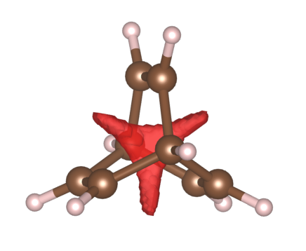
As another example, using the same procedure, we can clearly see that Bicylo[2,2,2]octane has a strong steric clash in the centre that pushes electrons out, indicated by the red regions.

The code to generate these results can be found: water_NCI.tar.gz; bicylo_NCI.tar.gz

To obtain these results:

run VASP using the files from vasp_input.tar.gz
rename the CHGCAR file from the single water molecule calculation to CHGCAR_single and put it and the CHGCAR for water dimer in the same folder.
run compare_RDG.py and analyze reduced_density_gradient.png.
run hessian.py and plot the color RDG using hess_color.vasp and rdg.vasp.

NOTE: The outpus are all in CHGCAR format so there will be a volume prefactor doted to the actual values. VESTA will automatically convert it back to is original values if it detect the name of the file starts with CHG.