Polar metals and hybrid Wannier functions

What is a “Polar metal”?

Polar metals are polar systems that are metallic, i.e. systems with Fermi energy crossing one or seveal bands across the Brillioun zone (Fermi crossing).

This behavior is unusual because the long range Coulomb interatcions which are usually considered to be the driving force of polar distortion is screened by having itenary electrons. Nevertheless, a whole lot of polar metals have been either experiementally identified or theoretically predicted.

The explaination of such behavior currently relies on the so-called “decoupled electron mechanism” (DEM) model. Proposed by Puggioni and Rondinelli in 2014, the DEM model states that the existence of polar metals relies on the coupling between the electrons at the Fermi level, and the phonons responsible for removing inversion symmetry to be weak. I.e. the origin of the conductivity and the origin of polar distortion are not related. For example, in some polar metal the conduction is constrain within a plane and the polarization is out-of-plane.

The usual Berryphase calculations are conducted by setting a string of k-points along a particular k direction ($k_z$) while sampling the other two k directions ($k_x$ and $k_y$). After obtaining the WCC along each string, average the results with respect to the k-point weight along $k_x$ and $k_y$.

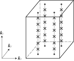
For polar metals that are conducting at one direction and insulating at another direction, people argues that one can calculate the polarization because the Berryphase (Wannier charge center) is still well defined in the out-of-plane direction $k_z$.

For a review of polar metals, I recommend the work of W. X. Zhou and A. Ariando.

Hybrid Wannier functions

Hybrid Wannier functions (HWFs) are Wannier functions that are only localized in one direction. It’s generated by Fourier transform (FT) the Bloch wavefunctions along one an only one direction. Because of this, it has dependencies on both two k-vectors ($k_a$ and $k_b$) that are perpendicular to the FT’ed direction and cell index along the FT’ed direction.

With Hybrid Wannier functions, we can calculate the Wannier charge centers (WCC) at each $k_a$ and $k_b$ points. The final polarization can be obtained by averaging WCCs over the $k_a$ and $k_b$ plane.

To get our heads around the HWFs, first, let’s remember the Wannier transformation (with Bloch subspace mixing using unitary matrix $U$):

\[\ket{\phi_{\vec R,n}} = \int_\text{BZ} e^{-i \vec k \vec R} \sum_m U^{\vec k}_{mn} \ket{\psi_{\vec k, m}} d\vec k \tag{1}\]

where $\phi$ is the Wannier functions, $\vec R$ labels the cell index, $n$ is the index of the Wannier functions, $m$ is the index of the Bloch WF $\psi$.

Inversely, one can obtain the Bloch functions from a set of Wannier functions by:

\[\ket{\psi_{\vec k',m'}} = \int_\text{all cell} e^{i \vec k' \vec R} \sum_n U^{\vec k *}_{nm'} \ket{\phi_{\vec R,n}} d \vec R \tag{2}\]

we can see this inverse transformation works because if we substitute $\phi$ in Eq. 2 with Eq. 1, we get:

\[\begin{aligned} \ket{\psi_{\vec k',m'}} &= \int_\text{all cell} e^{i \vec k' \vec R} \sum_n U^{\vec k *}_{nm'} \ket{\phi_{\vec R,n}} d \vec R \\ &= \int_\text{all cell} e^{i \vec k' \vec R} \sum_n U^{\vec k' *}_{nm'} \int_\text{BZ} e^{-i \vec k \vec R} \sum_m U^{\vec k}_{mn} \ket{\psi_{\vec k, m}} d\vec k d \vec R \\ &= \int_\text{BZ} \sum_n U^{\vec k' *}_{nm'} \left [ \int_\text{all space} e^{-i (\vec k' - \vec k) \vec R} d \vec R \right ] \sum_m U^{\vec k}_{mn} \ket{\psi_{\vec k, m}} d\vec k \\ &= \int_\text{BZ} \sum_n U^{\vec k' *}_{nm'} \delta(\vec k' - \vec k) \sum_m U^{\vec k}_{mn} \ket{\psi_{\vec k, m}} d\vec k \\ &= \sum_n U^{\vec k' *}_{nm'} \sum_m U^{\vec k'}_{mn} \ket{\psi_{\vec k', m}} \\ &= \sum_{nm} U^{\vec k' *}_{nm'} U^{\vec k'}_{mn} \ket{\psi_{\vec k', m}} \\ &= \ket{\psi_{\vec k', m'}} \end{aligned}\]

The formal definition of the hybrid Wannier functions is:

\[\begin{aligned} \ket{\phi_{R_c, k_a, k_b, n}} &= \int e^{-i k_c R_c} \sum_m U^{\vec k}_{mn} \ket{\psi_{\vec k, m}} d k_c \\ &= \int e^{-i k_c R_c} \sum_m U^{k_a,k_b,k_c}_{mn} \ket{\psi_{k_a,k_b,k_c, m}} d k_c \end{aligned} \tag{3}\]

In Eq. 3, we have only Wannier transformed one direction $k_c$ and left the other two directions $k_a$ and $k_b$ as individual parameters. This means we’ll get different WCCs along $c$ direction when choosing different $k_a$ and $k_b$.

We can also get this definition from a set of “fully transformed” Wannier functions $\phi_{\vec R,n}$:

\[\begin{aligned} \ket{\phi_{R_c, k_a, k_b, n}} &= \int e^{ik_a' R_a} \int e^{ik_b' R_b} \ket{\phi_{\vec R,n}} dR_a dR_b\\ &= \int e^{ik_a' R_a} \int e^{ik_b' R_b} \ket{\phi_{R_a, R_b, R_c ,n}} dR_a dR_b\\ \end{aligned} \tag{4}\]

Note that in Eq. 4, we no longer need $U^{\vec k *}_{nm’}$ like in Eq. 2, this is because we are going to keep using $n$ instead of switching to $m’$.

Eq. 4 also tells us that once we have the fully transformed Wannier functions, reverting to the hybrid form will not affect the Wannier charge center along the direction that hasn’t been inverse transformed (here $c$ direction). This is because mixing a Wannier function with its periodic images in cells that lie within $k_a$ and $k_b$ plane won’t change affect the position of said Wannier functions along the polarization direction $k_c$.

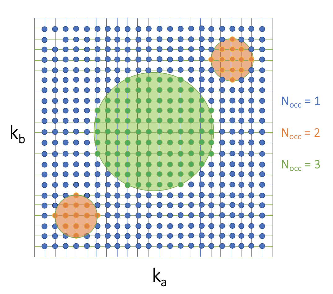
The good thing about $\ket{\phi_{R_c, k_a, k_b, n}}$ is that it depends on $k_a$ and $k_b$. This comes in handy for polar metals where bands crossover the Fermi level along $k_a$ and $k_b$ plane. For example, at $k_a$ and $k_b$ we have $n$ bands occupied, but at $k_a’$ and $k_b’$ we have $n+1$ bands occupied. If we want to calculate the polarization along $c$ axis, we need to calculate the WCCs along a string of k-points in $k_c$ direction at each set of $k_a$ and $k_b$ points.

To actually calculate the total polarization along the “non-conductive” axis, we first needs to divide the $k_a$ and $k_b$ plane by the number of bands occupied at each point.

For each subset, the WCCs can be obtained using Eq. 4. Specifically, we need to Wannierize the system with the number bands equal to the number of occupied bands in the subset. Note that this Wannierization process should be done with all k-points considered (including $k_c$) for each $k_a$ and $k_b$ set.

Specifically, for example, if I want to get the WCCs at the $k_a$ and $k_b$ where $n$ bands are occupied. I need to Wannierize the whole system by considering $n$ Wannier functions and get WCCs in three dimension, the $c$ component is the one that we are looking for. Then, moving to the next set of $k_a$ and $k_b$s where $n+1$ bands are occupied, I need to Wannierize the whole system again but with $n+1$ Wannier functions.

Once we’ve obtained the WCCs for each subset of the BZ, we can weight them by the k-points’ weight and obtain the finally WCCs along $c$ direction of the system.

Occupation controlled Berryphase method

For systems that are conductive only in the non-polarization directions, the work of Alessio Filippetti and co-workers suggested that the polarization can be decomposed into two components: the contributions from non-conductive bands and the contributions from the conductive electrons.

\[P_\text{total} = P_\text{non-conductive} + P_\text{conductive} \tag{5}\]

The non-conductive bands can be calculated using the usual Berryphase method as one can find a subset of bands that are occupied and are well seperated from other bands. For example:

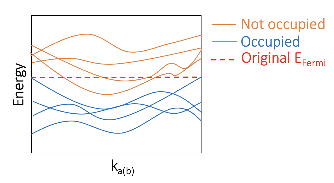
The usual Berryphase method (as implemented by VASP) uses default occupation obtained by the single-point calculations. However, this cannot be used for polar metals for the reason I’ve described. Instead, we need to constrain the occupation so that only only said subset of bands are occupied.

Practically, in VASP, one can set ISMEAR = -2 and FERWE to manually control the occupation of the bands. However, this is not natively allowed in LCALCPOL or LBERRY. Since LBERRY is more inline with what I’ve discussed here, I’ve modified LBERRY’s subroutine, (one can download the patch here). Just drop it in the the VASP distro and type patch -p0 < 2022-04-18-bp_occ.patch and compile away!

To use this occupation controlled Berryphase method, one has to do two steps:

Calculate the wavefunctions with a special KPOINTS.
Read wavefunctions from last step, constrain the occupation, calculate Berryphase related properties.

Note that for both steps, a special KPOINTS file is needed. The LBERRY module only work with k-points that are arranged such that the fast iterating index belongs to the k direction to be calculated. For example, if we need to calculate the polarization along $k_c$ axis, we need to have a KPOINTS file that looks like:

K-POINTS
216
rec
0 0
0 0.1
0 0.2
0 0.3
0 0.5
1 0 0
1 0 0.1
1 0 0.2
1 0 0.3
1 0 0.5

...

5 0.5 0.5

Also, for the second step, since we don’t want VASP to perform any kind of electronic energy minimization, we need to set ALGO = None and NELM=5.

The occupation constrain is to be set in the second step by ISMEAR and FERWE. Once ISMEAR=-2 is set, the occupation is read from either WAVECAR (if no FERWE is set) or FERWE. Since in our case we need all k-points to have a consistent occupation, we can use the following python script to generate the FERWE:

NKPTS = 216
NBAND_OCC = 93
NBAND_EMPT = 27
for ikpt in range(NKPTS):
    print(f"{NBAND_OCC}*1.0 {NBAND_EMPT}*0.0", end=' ')
print(' ')

In this example, we have a total of 216 k-points, and for each k-point, we have set the first 93 bands to be occupied and the last 27 bands to be unoccupied.

Finally, after the calculation, in the OUTCAR we can find:

e<r>_ev=(    -0.00000    -0.00000     0.00000 ) e*Angst
e<r>_bp=(     0.00000     0.00000   -32.13061 ) e*Angst

Total electronic dipole moment: p[elc]=(    -0.00000    -0.00000   -32.13061 ) e*Angst

ionic dipole moment: p[ion]=(   191.36251   110.48320   245.99999 ) e*Angst

Which is similar to the LCALCPOL results. To further obtain the polarization $P_\text{non-conductive}$, please refer to this post.

Next, we want to calculate the polarization of the polarization of the conductive electrons $P_\text{conductive}$. the work of Alessio Filippetti and co-workers suggested that it is possible to calculate the polarization by doing a planar average of the conduction charge density (can be obtained by band decomposed charge densities) along the non-conductive direction (or by taking the difference between charge densities calculated with different occupations). However, this only works if there are clear “near zero” points along the polarization direction that are more or less at the same place for both the polar and centro-symemtric phases, so that the charge center is well defined. Note that the existence of these “near zero” points is only coincidental and is not linked to the flatness of the bands along the polarization direction.

To give a concrete example, the conduction charge density of $\mathrm{Bi_5Ti_5O_{17}}$ goes down to around zero as seen in the work of Alessio Filippetti and co-workers:

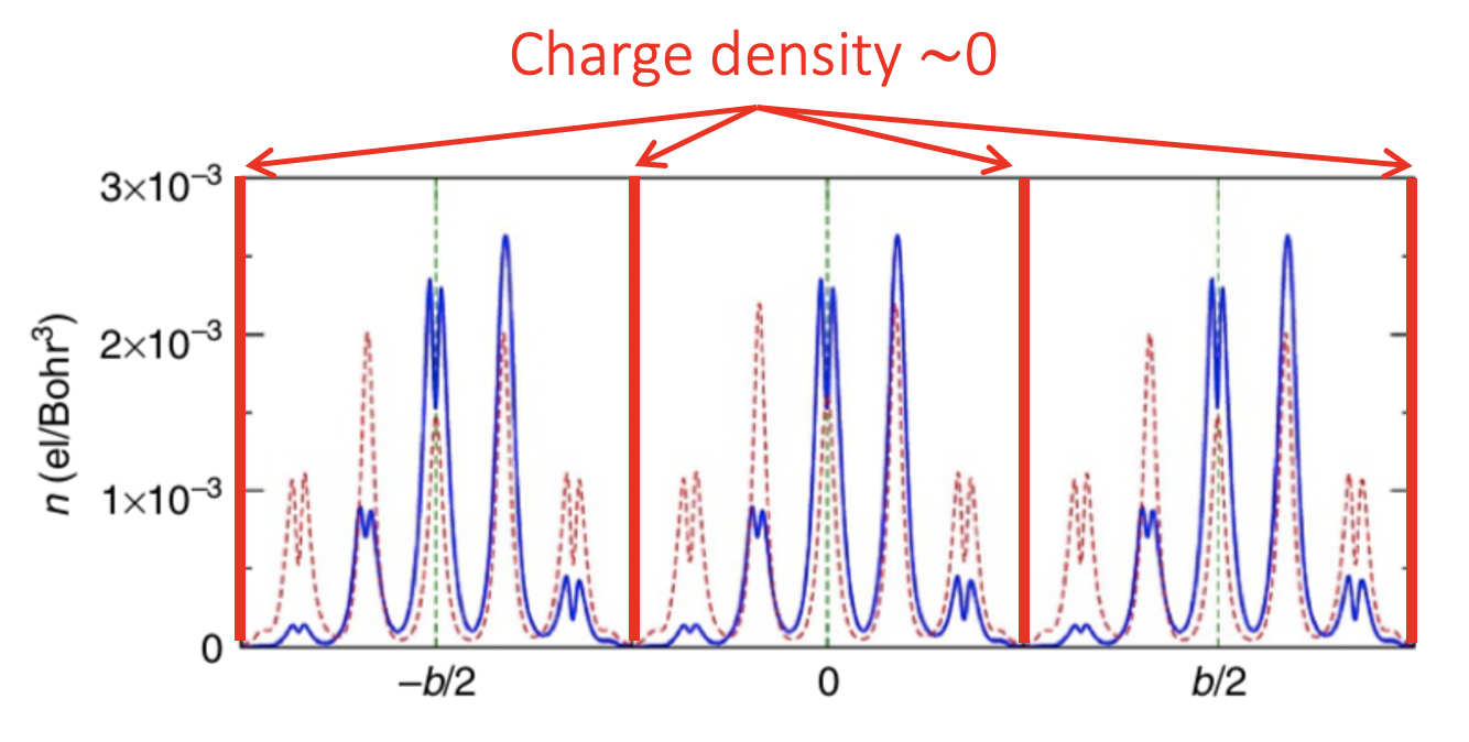
The charge center can be calculated by integrating the charge density over the well defined region (layer) with position as $\frac{\int_\text{layer} r \cdot \rho(r) dr}{\int_\text{layer} \rho(r) dr}$ and the dipole moment of such center can be easily obtained by $\int_\text{layer} r \cdot \rho(r) dr$.

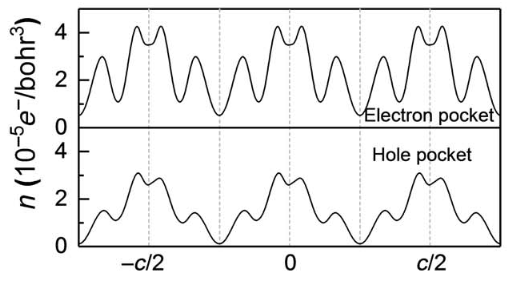
Pankaj Sharma and co-workers also used this method on $\mathrm{WTe_2}$ systems and they find that the electron pocket is more or less centro-symmetric so even though they have significant value on all points along $c$ axis, electron conduction channel doesn’t contribute to the polarization and only hole channel contributes:

This result is not that surprising. To understand it, we need to first consider Maximally Localized Wannier function (MLWF). What MLWF does is essentially finding the optimum band connections so that we can regroup the bands, get rid of the band crossing and obtain a set of wavefunctions that give rises to a well localized Wannier functions.

Now, not all Wannier functions contribute to the polarization (some of then have centers that don’t move much), which means some of the (re-organized) bands does not contribute to the polarization either. This is exactly the case of the electron pocket of $\mathrm{WTe_2}$.

Example

I’ve tried to reproduced the result of Pankaj Sharma and co-workers and the polarization I got is around $1.3 \mathrm{\mu C/cm^2}$.

I’ve put all the input files in a zip file for download: WTe2.