Searching for a shell
From velocity autocorrelation function to phonon DOS
The autocorrelation function is a cross-correlation function that shows the correlation of one signal (function) with a delayed version of it self. Essentially, It’s the phonoic analogue of the diagonal part of the Green’s function (for more details of quantum Green’s function, see ![]() this post and Eq. 11 of
this post and Eq. 11 of ![]() this post).
this post).
To derive the relation between velocity autocorrelation function and the phonon density of states, let us first start with the Fourier transforming the velocity of an atom $i$, $v_i(t)$.
The power spectrum (which tells us how the energy is distributed over the frequency) of this velocity function is:
Substitute $t-t’$ with $t’’$, the power spectrum can be re-written as:
Note that the exponential $e^{i\omega t}$ in Eq. 1 doesn’t contain a minus sign. This is just a difference in convention, if we put in the minus sign, then in Eq. 3 would become . However, this does not affect any of the following analysis.
Before moving on, let’s assume that harmonic approximation is valid (which, in theory, we should have zero-width phonon branches), the atomic displacement with respect to time can be written as:
where $s$ labels the phonon branch and $j$ is a composite index for the vibrations of atom $i$ on three spacial directions. Q is the amplitude of the vibration (with $\sqrt{\frac{1}{2} m_j}$ absorbed in) and $\omega$ is the frequency of the phonon mode.
With the time-dependent displacement derived, the time-dependent velocity can be expressed as:
Inserting Eq. 4 to Eq. 3, and notice we are now using $j$ instead of $i$ to incorporate three spacial dimensions, we get:
noting that, due to ![]() equipartition theorem, the total energy of an oscillator is $k_BT$ where $k_B$ is the Boltzmann constant and $T$ is temperature (there might be a factor of 2 missing here, but again, this won’t actually affect the final result as it merely acts as a scaling factor).
Since we can express the total energy as pure kinetic energy at the equilibrium position, we get:
equipartition theorem, the total energy of an oscillator is $k_BT$ where $k_B$ is the Boltzmann constant and $T$ is temperature (there might be a factor of 2 missing here, but again, this won’t actually affect the final result as it merely acts as a scaling factor).
Since we can express the total energy as pure kinetic energy at the equilibrium position, we get:
Substituting with $k_BT$, Eq. 5 becomes:
If we add contributions from all atoms (assuming there are $N$ atoms) in all three directions:
remember that the phonon DOS is expressed as , we can write phonon DOS as:
by the knowledge of Fourier transform of the time-dependent velocity function in Eq. 3, we get:
Remembering that the system is at its equilibrium state and the velocity signal is more or less periodic. For this reason, the following integral diverges:
Noting that the DOS function is a Dirac delta function, at $\omega = \omega_s$, the the DOS should indeed diverge. However, since we only care about the difference of the $\rho$ with different $\omega$s in our final plots, instead of using the integral above, we can re-write the integral as:
This expression can also be seen as a scaled velocity autocorrelation function:
Alternatively, we can re-normalize this autocorrelation function by doing something like:
Which, normalizes the maximum correlation to $1$ and we can get rid of the prefactor $dt’$.
This is what you see in, e.g. ![]() 10.1016/j.cpc.2011.04.019 or,
10.1016/j.cpc.2011.04.019 or, ![]() 10.1039/c8nr07373b.
10.1039/c8nr07373b.
Inserting Eq. 7 into Eq. 6, we get:
With Eq. 8, noting the decreasing nature of the velocity autocorrelation function so that the integral always converges, we see that if we have the knowledge of the velocity of each atom across a period of time (since we cannot do infinity, a we need to have a cut-off time for the integral), we can calculate the phonon density of states.
In practice, Eq. 8 should be rewrite in a discrete form as:
In summary, the Phonon density of states can be expressed as the Fourier transformed velocity autocorrelation function.
NOTE: I’ve ignored the $2\pi$ prefactor in all Fourier transformations.
Extension to periodic system
For periodic systems, the phonon bandstructure can also be interpreted as phonon DOS at each $k$ point. To obtain this “spectrum” function. we need to Fourier transform the velocity function with respect to the unit cell vectors. For example, lets say we have calculated a $\sqrt[3]{N}\times\sqrt[3]{N}\times\sqrt[3]{N}$ supercell (so that we have a total of $N$ unit cells):
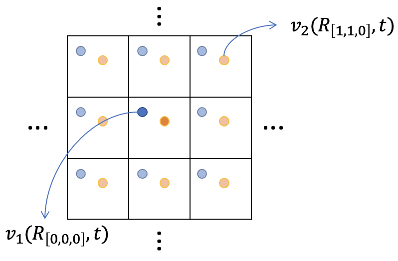
Here, we label the atoms in each cell with $j$ (again a composite label with three direction added) and the unit cell position is expressed as $\vec R$ so that the velocity of atom $j$ at cell $\vec R$ (in three direction) is:
Fourier (discrete) transform Eq. 9 with respect to $\vec R$, we get:
where we have $N$ unit cell in the supercell.
Using Eq. 10, we can express the phonon DOS at each $\vec k$ point as:
Here, the commensurate k-point can depends on supercell size. In other words, the larger your supercell is, the finner the k-points you can sample, and a better graph you’ll be able to get.
Physical explanation
Okay, the derivation is nice and easy, but what’s the physics behind?
Let’s consider a single atom that’s vibrating at its equilibrium position. Its velocity vs time can be plotted as:

The autocorrelation function $\int_{-\infty}^{\infty} v(t+t^{\prime})v(t^{\prime}) dt’$ of this velocity signal at different $t$ is:

We see that the autocorrelation function retains the periodicity of the orignal function. Such behavior will be reflected as a sharp peak in the Fourier spectrum.
For a more comprehensive understanding of the autocorrelation function, see ![]() this and
this and ![]() this post.
this post.
See it in action
Download: ![]() code
code
Now it’s time to try it out! Using water molecule (so that I don’t have to deal with the k-depenedence of periodic systems, which requries a huge super cell to achieve sufficient sampling) as an example, we are going to compare the phonon frequencies calculated with DFT (DFPT) to the ones that we have obtained using our MD mtehod.
The three Raman active mode from our DFT calculation have frequencies: 47 THz($a_1$), 111 THz($b_2$), 114 THz($a_1$), comparable to ![]() the experiemental values.
the experiemental values.
With a molecular dynamic calculation of a single water molecule thermalized at 300K, we get the following plot:
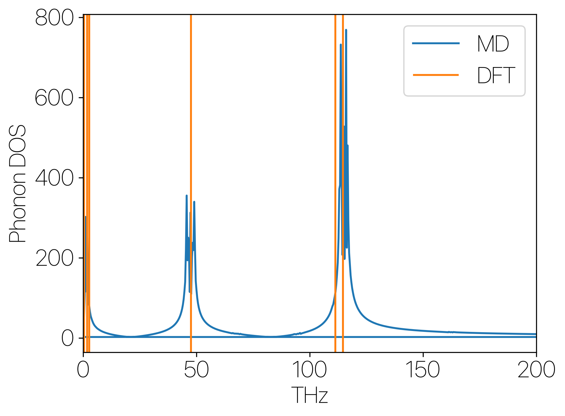
Okay, it works!!