Using Wannier Charge center to calculate Ferroelectric polarization

Background

According to “the Modern theory of polarization”, in a continous-k formulation, the polarizatin $\mathbf{P}_\text{electron}$ value is $- f e / (2 \pi)^3$ times the sum of valence-band Berry phase. On another note, Wannier charge center can be conveniently linked to the Berryphase of valence band via a Fourier transformation. Thus, we should be able to calculate the ferroelectric polarization using Wannier interpolation of Bloch bands.

Objectives

To calculate the polarization value of $\text{BaTiO}_\text{3}$ , compare it with the Berryphase one.
To give a rough idea of how periodicity affect the calculation of the ferroelectric polarization.
To get familiar with the VASP2WANNIER90 interface

Structure(s)

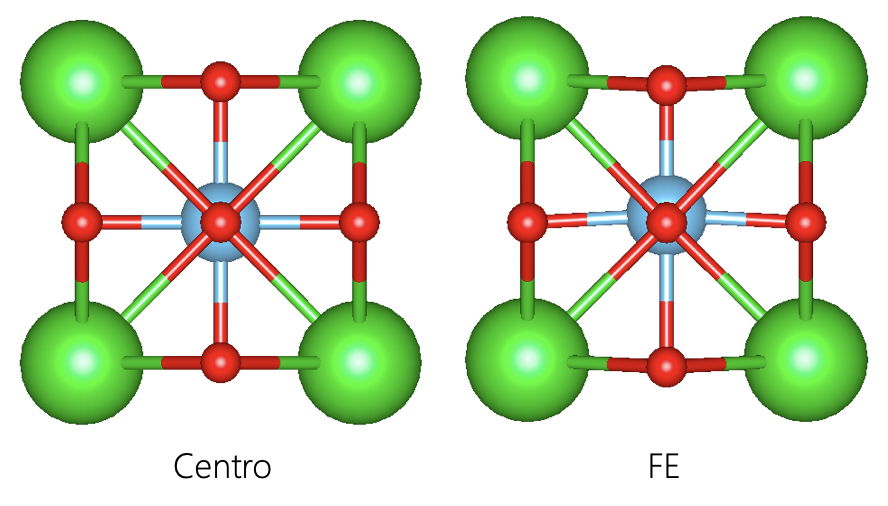
We need both centro symmetric and non-centro Ferroelectric structure.

Berryphase method

To get polarization value using VASP, just add the following line to your SCF(static) calculation’s INCAR:

LCALCPOL=.T.

In the OUTCAR file, you will find a block like the following:

     CALCP:  cpu time   11.0656: real time   11.0798

            Ionic dipole moment: p[ion]=(     0.00000     0.00000   -11.57420 ) electrons Angst

 Total electronic dipole moment: p[elc]=(    -0.00000    -0.00000    -1.68410 ) electrons Angst

For the result, I refer back to one of my previous post:

By varying the atomic displacement from the centrosymmetric phase (CENT) to ferroelectric one (FE). VASP produce a series of ionic and electronic contribution to the total dipole moment.

Image	Ion (elect*A)	Electron (elect*A)
0 (CENT)	+00.00000	+0.00000
1	-12.01278	-0.29138
2	-11.92507	-0.58047
3	-11.83735	-0.86532
4	-11.74963	-1.14461
5	-11.66192	-1.41757
6 (FE)	-11.5742	-1.68399

we can easily calculate its ionic dipole moment at centrosymmetric phase should be -12.09 elect*A.
After figuring out which value is clearly wrong, we can now proceed to calculate total polarization:

Total ionic contribution = 0.5258 elect*A
Total electronic contribution = -1.68399 elect*A
Total dipole moment = -1.15819 elect*A
Volume = 64.35864801 A^3

Total polarization = 0.288293871 C/m^2

Wannier charge center method

In this section, I will introduce the usage of VASP2WANNIER90 interface as well as a general method to construct the valence band’s Wannier functions.

Wannier functions are a set of localized functions generated using Fourier transformation of periodic Bloch functions.
We only use valence bands to generate Wannier functions so that the square of it can represent the charge density.
Each Wannier function “corresponds” to an energy band, hence, each Wannier function is occupied by 2 electrons (or 1 if we treat each spin channel separately).

Fat band analysis

We need fat band analysis in order to get a sense of how our valence band are composed. Here, for the sake of simplicity, I’ll skip it and the reader should feel free to to calculate these on their free time.

The result should coincide with our chemical intuition. From the electron configurations, we can see that:

Element	Electron configuration	Valency	Number in the unitcell
$\text{Ti}$	3s(2) 4s(1) 3p(6) 3d(3)	+4	1
$\text{Ba}$	5s(2) 6s(2) 5p(6)	+2	1
$\text{O} $	2s(2) 3p(4)	-2	3

which means, our valence bands are composed by:

Ti         : 3s(2) 3p(6)
Ba         : 5s(2) 5p(6)
O          : 2s(2) 3p(6)

and the ionic charge of each atom is:

Ti         : 12
Ba         : 10
O          : 6

Setting up `Wannier90.win`

VASP2WANNIER90 interface requires following parameters to run(at minimum):

num_wann        =  20

begin projections
Ba:s,p
Ti:s,p
O:s,p
end projections

Here, I used $\text{Ba}$’s $s$ and $p$ orbitals, $\text{Ti}$’s $s$ and $p$ orbitals and $\text{O}$’s $s$ and $p$ orbitals as initial projection.

Since we have a set of isolated valence bands, we can exclude the conduction bands by adding:

num_bands = 20
exclude_bands = 21-24

Other information such as cell vectors, atom’s positions, k-points can be written automatically by VASP.

Furthermore, I added num_iter = 0 to use projection only scheme.

After written wannier90.win file, add the following line:

LWANNIER90 = .T.

to your INCAR and run it. VASP will produce wannier90.mmn, wannier90.amn, wannier90.eig files.

Then run WANNIER90 by:

wannier90.x wannier90

and it will generate wannier90.out file. Near the end of that file, there should be a block that look like the following:

Final State
 WF centre and spread    1  ( -0.000000, -0.000000,  0.003016 )     1.21085811
 WF centre and spread    2  (  0.000000,  0.000000, -0.003455 )     1.28081902
 WF centre and spread    3  ( -0.000000,  0.000000, -0.003910 )     1.28327685
 WF centre and spread    4  (  0.000000, -0.000000, -0.003910 )     1.28327685
 WF centre and spread    5  (  1.997250,  1.997250,  2.107985 )     0.80169939
 WF centre and spread    6  (  1.997250,  1.997250,  2.071553 )     0.51270417
 WF centre and spread    7  (  1.997250,  1.997250,  2.073947 )     0.51094776
 WF centre and spread    8  (  1.997250,  1.997250,  2.073947 )     0.51094776
 WF centre and spread    9  (  1.997250,  1.997250,  3.904794 )     0.80411119
 WF centre and spread   10  (  1.997250,  1.997250,  3.838697 )     1.37763989
 WF centre and spread   11  (  1.997250,  1.997250,  3.826994 )     1.31815348
 WF centre and spread   12  (  1.997250,  1.997250,  3.826994 )     1.31815348
 WF centre and spread   13  (  1.997250, -0.000000,  1.970000 )     0.80517833
 WF centre and spread   14  (  1.997250,  0.000000,  1.969097 )     1.33523984
 WF centre and spread   15  (  1.997250,  0.000000,  1.973544 )     1.34961978
 WF centre and spread   16  (  1.997250,  0.000000,  1.975866 )     1.41185754
 WF centre and spread   17  ( -0.000000,  1.997250,  1.970000 )     0.80517833
 WF centre and spread   18  (  0.000000,  1.997250,  1.969097 )     1.33523984
 WF centre and spread   19  (  0.000000,  1.997250,  1.975866 )     1.41185753
 WF centre and spread   20  (  0.000000,  1.997250,  1.973544 )     1.34961977
 Sum of centres and spreads ( 23.967000, 23.967000, 39.493663 )    22.01637893

those three data between parentheses are the Wannier Charge Centers:

\mathbf{R}_{i} = \langle \psi_{i} | \mathbf{r} | \psi_{i} \rangle

And that, my friend, is all the technical details you need to know to calculate the Wanneir charge centers.

According to “the modern theory of polarization”, the macroscopic polarization can only be obtained by subtracting the centrosymmetric phase’s dipole moment from the Ferroelectric one. Here, I’ll do a little trick to circumvent this and eventually show you how everything fits back together.

Calculate the polarization without centrosymmetric phases

The centrosymmetric phase can be safely ignored when its polarization equals to ZERO with a huge asterisk that the ferroelectric phase should still be on the same “polarization branch” as the centrosymmetric phase.

To calculate the electronic contribution to the polarization, just sum each Wannier Charge Centers and then multiply if by a spin-degenerate factor $2$:

\mathbf{P}_\text{electron}=2 * \sum_{i} \mathbf{R}_{i}

To calculate the ionic contribution to the polarization, first find each ions core charges (positive), then multiply the atomic position (here, along z axis) by it and sum up the data:

\mathbf{P}_\text{ion}=\sum_{I} C_{I} \mathbf{R}_{I}

since $\mathbf{r}$ and $\mathbf{R}$ are vectors, in order to get the total polarization, we have to do this on three Cartesian axes and then add them up using vector summation. Here, we only care about the polarization at Z axis, so I’ll just ignore other axes’ contributions. My results are as follow (note the minus sign in Ionic part is due to electrons having negative charge):

Ionic dipolemoment(elect*A):     -72.0768  
electric dipolemoment(elect*A):   78.9873
Total dipolemoment(elect*A):      06.9105
Volume(A^3):                      64.3586
Total polarization(C/M^2):       -01.7201

where the ionic dipolemoment is calculated by:

-(12\times2.0743+0\times10+6\times3.9306+6\times1.9668+6\times1.9668) = -72.0768

This value is drastically large than the one we get using Berryphase method so there must be something wrong!

Indeed, here, we encountered the so-called polarization quantum. (Remember that huge asterisk saying the ferroelectric phase shoud be on the same branch as the centrosymmetric phase? if they are not, the difference is this “polarization quantum”)

\mathbf{P}_\text{quantum}=N \cdot \text{Lattice parameters}

Where N equals to some integer number that represent the number of electron get involved.

Taking a closer look at our structures, the FE one has one oxygen at ~$3$ Å while it goes to $0$ Å in the centrosymmetric phase (see picture below). An atom moving $3$ Å during phase transition is generally speaking not possible!

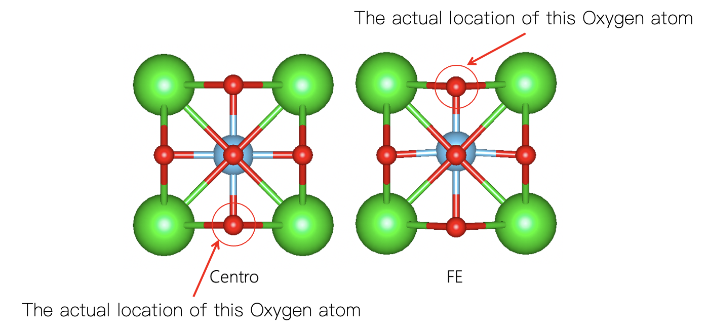
Intuitively, one may think “OK, thats alright, we have periodic boundary, so we only have to move this atom up-wards to the boundary.” Yes, this is indeed the case, but our method cannot deal with this, and that is why the polarization quantum is always linked with the lattice parameters and the polarization curve (displacement vs polarization) is multi-valued.

To solve this, we can simply subtract one lattice parameter Z from the atomic position as well as the corresponding Wannier Charge Centers, we get (again, note the minus sign in Ionic part is due to electrons negative charge sign):

Ionic dipolemoment(elect*A):     -47.8758  
electric dipolemoment(elect*A):   46.7193
Total dipolemoment(elect*A):     -01.1565
Volume(A^3):                      64.3586
Total polarization(C/M^2):        00.2879

where the ionic dipolemoment is calculated by:

-(12\times2.0743+0\times10+6\times(-0.1029)+6\times1.9668+6\times1.9668) = -47.8758

This way, our polarization calculated via Wannier functions is almost identical to our Berryphase’s result.

Calculate the polarization with centrosymmetric phases

If we stick with the method described above, finding what went wrong can be tedious if not impossible for larger systems, especially when you are confused about which Wannier function belongs to which atom.

Don’t be afraid! There is another way of dealing with the polarization quantum. Remember what we did to the centrosymmetric phase? Yep, we ignored it because its polarization is zero and zero doesn’t seem to be that interesting. However, even though the overall dipole moment of the centrosymmetric phase is zero, each orbital associated with atoms still have Wannier charge centers and we can use those Wanneir charge centers as a “homing beacon” to determine which cell should the same Wannier charge centers located in the ferroelectric phase.

The exact way of doing this is by finding the shortest route to move from the ferroelectric phase’s Wannier charge center to centrosymmetric phase’s Wannier charge centers.

I’ll leave this to the reader to use this method to calculate the polarization value.

WARNING The sign convention for the ionic part is very important. Please, for the love of god, remember change dot the dipole moment of each structure’s result with a minus sign and ADD it to the electronic part (so that they are both in elect * A). And remember to flip the sign of the final result (in C/M^2).

Conclusion

The calculation of the macroscopic electric polarizations can have many pitfalls, and almost all of them are related to the polarization quantum. So, check your structures, make sure no ions jump over the boundary!

Input

I’ve put all input file in a zip file for download: VASP.