Real-space Wannier Orbital Population analylsis

References

Referenc: https://pubs.rsc.org/en/content/articlepdf/2010/cp/b918890h
Code repo: https://github.com/Chengcheng-Xiao/WOOPs

Wannier function $\phi_n$ sitting in cell $\mathbf{R}$ is defined as

\phi_{\mathbf{R},n}(\mathbf{r}) =\frac{V}{(2\pi)^3} \int_\text{BZ} e^{-i \mathbf{k}. \mathbf{R}} \sum_m U^{\mathbf{k}}_{mn} \psi_{\mathbf{k}, m} (\mathbf{r}) d\mathbf{k},

where $\psi_{\mathbf{k}, m}$ is Bloch states at $\mathbf{k}$ point and band number $m$, $U$ is a unitary matrix that mixes the Bloch states. The constraint here is that $U$ needs to be square, meaning the number of $m$ needs to be the same as $n$.

The choice of $m$ determines the properties of Wannier functions (i.e., which subset of bands they describe). One can construct molecular orbital-like Wannier functions by constraining $m$ to be only the occupied states. Or, atomic orbital like Wannier functions can be constructed by setting $m$ to also include the anti-bonding like states in the unoccupied manifold.

The main Goal of WOOP and WOPP is to decompose Wannier charge and dipole from molecular-like Wannier orbitals (MO) using a set of atomic-like Wannier orbitals (AO).

MO to AO decomposition

First, we project MOs ($W$) on to a set of AOs($\phi$) to get the projection coefficients ($C$) by solving a set of coupled equations

\sum_{j=1}^N S_{mj} C_{jI} = \braket{\phi_m|W_I}

Here, unlike what Joydeep et al. did, the AOs and MOs are all Wanneir functions from the same set of Bloch functions (MOs are restricted to be occupied Bloch states only and AO uses some empty bands). This means that the AOs forms a orthonormal basis, i.e., $S$ is identity. Because of this, the projection coefficients $C$ are simply

C_{mI} = \braket{\phi_m|W_I}

Again, because the AOs and MOs are all Wanneir functions from the same global set of Bloch functions, the underlying basis (Bloch states) is the same, and the $U$ matrix for the MOs can be zero-padded to be the same shape as $U$ matrix for the AOs. Hence,

C_{m,I} =\braket{\phi_m|W_I} =\int_\mathbf{k} \sum_n U^{\mathrm{AO}*}_{nm} U^{\mathrm{MO}}_{nI} e^{i\mathbf{k}.(\mathbf{R}_m-\mathbf{R}_I)} d\mathbf{k}.

Note that here $I$ and $m$ are composite indices that also specifies which cell does these Wannier functions sits $R_m$ and $R_l$.

Wannier Orbital Overlap Population

With $C$ calculated, the charge of a Wannier functions carries can be expressed as

\rho_I = \braket{W_I | W_I},

With $C$ calculated, $\rho^I$ can be decomposed into the Wannier Orbital Overlap Population (WOOP) $B_{lm}^I$

B_{lm}^I = C_{Il} S_{lm} C_{Im} = \delta_{l,m} C_{Il} C_{Im}.

Here, because AOs form an orthonormal basis, $B^I$ is a diagonal matrix. Remember MOs $W$ describes only the occupied bands, the total charge of the system can be represented as

\rho = \sum_I \braket{W_I | W_I} = \sum_{I,l,m} B_{lm}^I = \sum_{I} \mathrm{Tr}(B^I).

Wannier Orbital Position Population

Similar to Wannier charge, the Wannier charge centre (WCC)

\braket{\mathbf{r}}_I = \braket{W^I |\mathbf{r}| W^I}

can be decomposed into the Wannier Orbital Position Population (WOPP) $D_{lm}^I$,

D_{lm}^I = C^*_{Il} \phi^*_l \mathbf{r} \phi_m C_{Im} = C^*_{Il} \left[ \phi^*_l \mathbf{r} \phi_m\right] C_{Im} = D_{Il} \mathbf{r}_{lm} C_{Im}

and $\sum_{l,m} D_{lm}^I$ should give $\braket{\mathbf{r}}_I$.

BEC decomposition

The electric contribution to the dipole moment can be obtained from WCC

\mathbf{d}^\mathrm{elect.} = -2\sum_{I\in\text{occ.}} \braket{\mathbf{r}}_I =-2\sum_{I\in\text{occ.}} \sum_{l,m} D_{lm}^I,

where the factor $-2$ comes from the fact that electron has negative charge and each Wannier function can be occupied by two electrons. Note that here $\mathbf{d}$ has the unit of abs(electron)Å. The total dipole moment is:

\mathbf{d} = \mathbf{d}^\mathrm{elect.} + \mathbf{d}^\mathrm{ion.}

where $\mathbf{d}^\mathrm{ion.}$ is the ionic contribution.

For periodic system, the centro-symmetric contribution needs to be subtracted from teh

\mathbf{d}= \mathbf{d}_\mathrm{FE} - \mathbf{d}_\mathrm{Centro.}

We are now ready to derive the Born effective charge (BEC) tensor $Z$

Z_{\kappa,ij} = \frac{\partial \mathbf{d}_i}{\partial \mathbf{u}_{\kappa, j}}

where $\mathbf{u}_{\kappa, j}$ denotes the distortion of atom $\kappa$ along direction $j$, and $\mathbf{d}_i$ is the induced change in the total dipole moment.

Assuming the ferroelectric distortion is within the linear regime, the derivative can be discretised as

Z_{\kappa,ij} = \frac{\mathbf{d}^\mathrm{elect.}_\mathrm{FE} - \mathbf{d}^\mathrm{elect.}_\mathrm{Centro.} }{\mathbf{u}_{\kappa, j}} + Z^\mathrm{ion}

We can express $\mathbf{d}$ with WOPP $D$

\begin{aligned} Z_{\kappa,ij} &= \sum_{I\in\text{occ.}} \sum_{l,m} Z^\mathrm{elect.}_{\kappa,ij} + Z^\mathrm{ion} \\ &=\frac{\left[ -2\sum_{I\in\text{occ.}} \sum_{l,m} D_{lm}^{I,\mathrm{FE}} - -2\sum_{I\in\text{occ.}} \sum_{l,m} D_{lm}^{I,\mathrm{CENT}} \right]_i}{\mathbf{u}_{\kappa, j}} + Z^\mathrm{ion}, \end{aligned}

and $Z^\mathrm{elect.}_{\kappa,ij}$ can be further decomposed as

Z^\mathrm{elect.,I}_{\kappa,ij,lm}= -2 (D_{lm}^{I,\mathrm{FE}}-D_{lm}^{I,\mathrm{CENT}})_i/{\mathbf{u}_{\kappa, j}}

where depending on which atom $l$ and $m$ belongs to, we can identify specific contributions to the BEC and gain more insights into the origin of ferroelectrics.

Test case: PbTiO3

All files an instruction to run can be found: PTO_WOOPs.tar.gz

The band features of PbTiO3 looks like 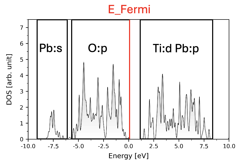In this case, for MO, all Bloch bands between -10 and 0eV are used and projection are made onto Pb’s s-orbital and O’s p-orbitals. For AO, all Bloch bands between -10 and 9eV are used and projection are made onto Pb’s s-orbital, O’s p-orbitals, Ti’s d-orbitals and Pb’s p-orbitals.

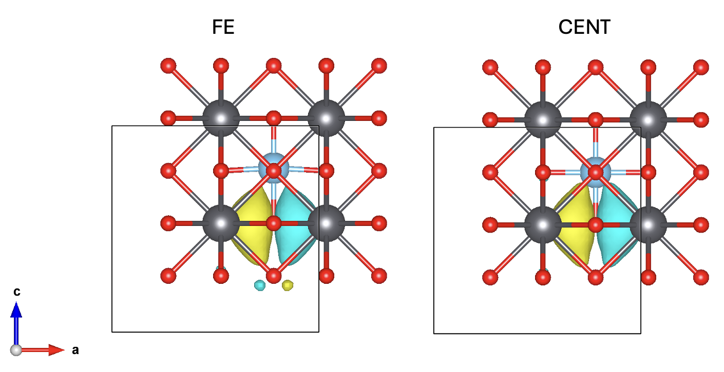
With our Wannierzation strategy set, we Wannierized both centrosymmetric and Ti-displaced PTO structures.

First of all, let’s take a look at the Wannier centres of both centrosymmetric and Ti-displaced PTO:

---------------------------------------------------------------------
ELECTRONIC PART

Centro symmetric: 
WF centre and spread    1  ( -0.000000, -0.000000, -0.000000 )
WF centre and spread    2  (  1.944478,  1.944478,  0.000000 )
WF centre and spread    3  (  1.944478,  1.944478,  0.000000 )
WF centre and spread    4  (  1.944478,  1.944478,  0.000000 )
WF centre and spread    5  (  0.000000,  1.944478,  1.944478 )
WF centre and spread    6  (  0.000000,  1.944478,  1.944478 )
WF centre and spread    7  (  0.000000,  1.944478,  1.944478 )
WF centre and spread    8  (  1.944478,  0.000000,  1.944478 )
WF centre and spread    9  (  1.944478,  0.000000,  1.944478 )
WF centre and spread   10  (  1.944478,  0.000000,  1.944478 )
Sum of centres and spreads ( 11.666867, 11.666867, 11.666867 )

Ti-displaced
WF centre and spread    1  ( -0.000000, -0.000000, -0.002362 )
WF centre and spread    2  (  1.944478,  1.944478, -0.031280 )
WF centre and spread    3  (  1.944478,  1.944478, -0.076180 )
WF centre and spread    4  (  1.944478,  1.944478, -0.076180 )
WF centre and spread    5  (  0.000000,  1.944478,  1.947213 )
WF centre and spread    6  (  0.000000,  1.944478,  1.955115 )
WF centre and spread    7  (  0.000000,  1.944478,  1.955985 )
WF centre and spread    8  (  1.944478,  0.000000,  1.947213 )
WF centre and spread    9  (  1.944478,  0.000000,  1.955985 )
WF centre and spread   10  (  1.944478,  0.000000,  1.955115 )
Sum of centres and spreads ( 11.666867, 11.666867, 11.530624 )

diff in z [using wannier centre] : -2*(11.530624)- -2*(11.666867) = 0.272486 electron*A

---------------------------------------------------------------------
IONIC PART

CENT                    X          Y          Z          Normal charge
Atom:     Ti  Position: 1.9444779, 1.9444779, 1.9444779  4
Atom:     Pb  Position: 0.0000000, 0.0000000, 0.0000000  4
Atom:     O   Position: 1.9444779, 1.9444779, 0.0000000  4
Atom:     O   Position: 0.0000000, 1.9444779, 1.9444779  4
Atom:     O   Position: 1.9444779, 0.0000000, 1.9444779  4
total_moment            23.333734, 23.333734, 23.333734


FE                      X          Y          Z          Normal charge
Atom:     Ti  Position: 1.9444779, 1.9444779, 2.0444779  4
Atom:     Pb  Position: 0.0000000, 0.0000000, 0.0000000  4
Atom:     O   Position: 1.9444779, 1.9444779, 0.0000000  4
Atom:     O   Position: 0.0000000, 1.9444779, 1.9444779  4
Atom:     O   Position: 1.9444779, 0.0000000, 1.9444779  4
total_moment            23.333734, 23.333734, 23.733735

diff in z [using ionic position] : (23.733735)-(23.333734) = 0.4 electron*A

With both the electronic part and ionic part of the dipole moments, the final total dipole moment is

Total polarization: (P(ION)+P(ELECT))/(cell_volume) = 0.672486 electron*A / 58.8165 A^3

With WOPP, we can check if it reproduces the WCCs using the following codes

import h5py
import numpy as np

#READ
dist = 0.1 #\Angstrom

opf = h5py.File("WAN_MAT_FE.h5", "r")
WOPP_FE = opf['WOPP'][:]
opf.close()

opf = h5py.File("WAN_MAT_CENT.h5", "r")
WOPP_CENT = opf['WOPP'][:]
opf.close()

# reproduce Wannier centers
# FE
WCC_FE = []
for i in range(10):
    WCC_FE.append([np.sum(WOPP_FE[0,i]).real,np.sum(WOPP_FE[1,i]).real,np.sum(WOPP_FE[2,i]).real])
    print(np.sum(WOPP_FE[0,i]).real,np.sum(WOPP_FE[1,i]).real,np.sum(WOPP_FE[2,i]).real)
# CENT
WCC_CENT = []
for i in range(10):
    WCC_CENT.append([np.sum(WOPP_CENT[0,i]).real,np.sum(WOPP_CENT[1,i]).real,np.sum(WOPP_CENT[2,i]).real])
    print(np.sum(WOPP_CENT[0,i]).real,np.sum(WOPP_CENT[1,i]).real,np.sum(WOPP_CENT[2,i]).real)

and we get

-----------------------------------------------------------------
FE
WF centre 0.005457029803540602  0.0054570297773970195 0.004255264833346661
WF centre 1.9447789431382763    1.9447789431340554   -0.030624440288172627
WF centre 1.937768439471597     1.941449120137218    -0.07843681899596507
WF centre 1.941449120219155     1.9377684394679062   -0.0784368191151973
WF centre 0.0009242643140386245 1.9417406120320475    1.9409903884146886
WF centre 0.0005663412429231772 1.945921535413768     1.9558120272283457
WF centre 0.0009764261688857814 1.9379821644723874    1.9536919910367032
WF centre 1.9417406119706437    0.0009242638801744313 1.9409903883589483
WF centre 1.9379821645546589    0.0009764261274046967 1.953691990879517
WF centre 1.9459215354391581    0.0005663413290268558 1.9558120270123225

-----------------------------------------------------------------
CENT
WF centre 0.0056661899212342255  0.005666189903008093   0.00565587885084541
WF centre 1.9449951440216728     1.9449951440185393     0.0015071280882127907
WF centre 1.9379484431461589     1.941643063427853      0.0009849934888696372
WF centre 1.941643063449559      1.9379484431173157     0.000984993502376968
WF centre 0.0009897481803453805  1.9416310929621265     1.9379595711051945
WF centre 0.00024483995096022306 1.9460389254623531     1.9448450213758401
WF centre 0.0009970042526089658  1.937943962970781      1.9416336872564393
WF centre 1.9416310929120248     0.000989748185270458   1.9379595709880377
WF centre 1.937943962977724      0.0009970042511571067  1.9416336873355562
WF centre 1.9460389254168549     0.00024484000013661345 1.9448450213530668

we see that the total dipole moment is properly reproduced and the total dipole moment along z-axis calculated using WOPP is:

Total_dipole 0.28052710795980484

Taking a look at completeness.txt generated from running woops.py, we also find all MOs are perfectly reproduced with AOs hence they are normalised and the total number of charge is conserved.

With this script get_z.py (which requires WAN_MAT_CENT.h5 WAN_MAT_FE.h5), the BEC is decomposed using WOPPs.

Focusing on MO_2:

The WOPP decomposition of $Z$ of MO_2 is:

Atom: 2  MO: 2
CT: 1.8900887213008697
LP: -0.0009889066762047358
COV: -0.28750406100028203
NC: -0.04753727747447927

where CT is charge transfer, LP is local polarizability, COV is covalency and NC is non-local contribution (see Fig.3 of reference).

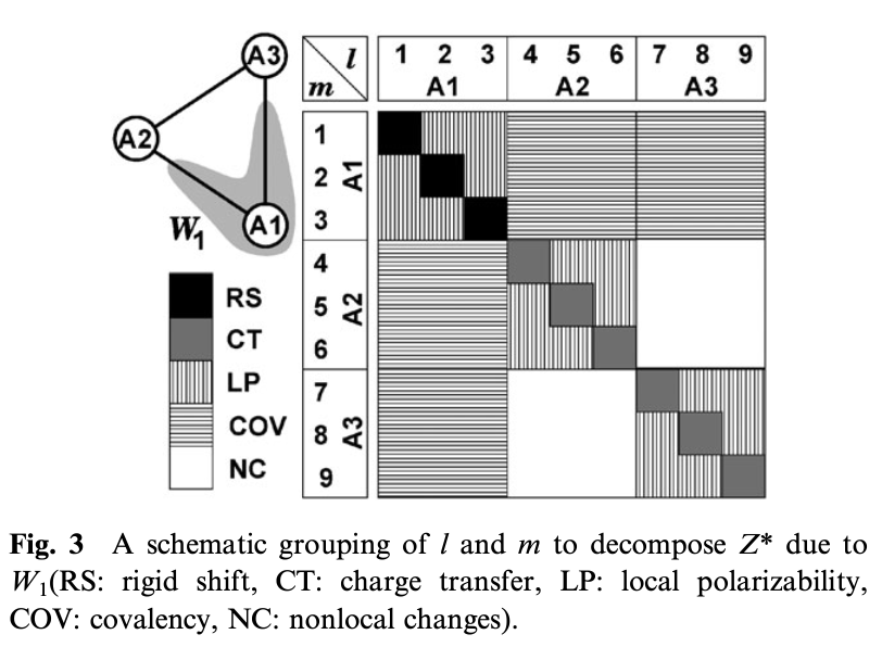
we see that indeed as described in the reference, the major contribution comes from charge transfer from O to Ti.