Orbital decomposition of magnetic anisotropy energy using VASP

The full Hamiltonian including the spin-orbital coupling term can be written as:

where the SOC strength $\lambda(r)$ is:

and $r$ is the distance to the atomic core, $V$ is the all-electron potential near core region (in the PAW formalism).

For 3d states, the integrated value of $\lambda(r)$ is about 30 meV, comparing to the usual hopping parameter, this energy is negliable and the SOC term could be treated as perturbation to $H_0$.

Using perturbation theory, the first order energy correction is:

where $\ket{n}$ are the wavefunctions (eigenvectors) to the original Hamiltonian $H_0$. Since the diagonal part of $H_\mathrm{SO}$ is zero (you can check this using the wanSOC pakcage), $E^{(1)}_\mathrm{SO}$ is evaluated to be zero.

The second order energy correction is:

where $o$ denotes the occupied states and $j$ sums over all states. However, when $j$ is also an occupied state, the two terms arising from the exchange of $o$ and $j$ cancels each other:

Because of this, the interaction can only happen between occupied ($o$) and empty states ($u$):

If we also include spin degrees of freedom, we could have two types of coupling:

• The coupling between occupied down(up) and unoccupied down(up) states: $E_{--}$ ($E_{++}$).
• The coupling between occupied up(down) and unoccupied down(up) states: $E_{+-}$ ($E_{-+}$).

The total SOC energy is approximately (ignoring third order an up terms) equal to the sum of these two contributions:

where:

Depending on the magnetization axis, assuming that there are no mixing in the orbital part, we can write the spin part of the spinor wavefunction as:

• magnetization along x axis: $\frac{1}{2}\begin{pmatrix} 1 & -1 \end{pmatrix}$
• magnetization along z axis: $\begin{pmatrix} 0 & 1 \end{pmatrix}$

For example, inserting these into $\braket{o^-\vert\hat{\sigma}\hat{L}\vert u^-}$, we have:

As a result, the energy difference bewteen the spin polarized $E_{–}$ terms with spin aligned along $x$ and $z$ axes is:

Similarly, we can calculate the energy difference with $E_{+-}$ as,

Combining the energy difference of up-up, up-down, down-down and down-up together, we get the total MAE as:

The matrix elements of $L_z$, $L_x$ and $L_y$ can be easily generated using wanSOC package. For example, the matrix elements of $L_x$ under the basis of $d$ orbitals can be generated using the following code:

from __future__ import print_function
import numpy as np
from wanSOC.basis import *
from wanSOC.io import *
from wanSOC.helper import *
from wanSOC.hamiltonian import *

basis = creat_basis_lm('d')

Lz = MatLz(basis)
Lp = MatLp(basis)
Lm = MatLm(basis)
# generate transformation matrix from complex to real spherical harmonics
trans_L = trans_L_mat(orb)
# apply transformation
Lz = np.dot(np.dot(trans_L.H, Lz),trans_L)
Lp = np.dot(np.dot(trans_L.H, Lp),trans_L)
Lm = np.dot(np.dot(trans_L.H, Lm),trans_L)

Lx = (Lp+Lm)/2

print(np.array_repr(Lx, max_line_width=80, precision=6, suppress_small=True))

For real systems, each Kohn-Sham orbital can be described using a linear combination of atomic orbitals near the core regions. Hence, the contribution of these Kohn-Sham wavefunctions to the MAE can be easily decomposed into the atomic contributions using projection method. For example:

          dz2,    dxz,    dyz,dx2-dz2,    dxy
|\psi> = [0.0,    0.5,    0.5,    0.0,    0.0] 

And $\braket{\psi\vert L\vert\psi}$ can then be calculated. As a result, the MAE can be decomposed into the contributions from the molecular orbtial.

Using this procedure, I’ve reproduced Fig. 2(b) of 10.1038/s42005-018-0078-4 which shows the $\braket{L_z}$ and $\braket{L_x}$ of the d-orbital related molecular orbitals of a Ir dimer.

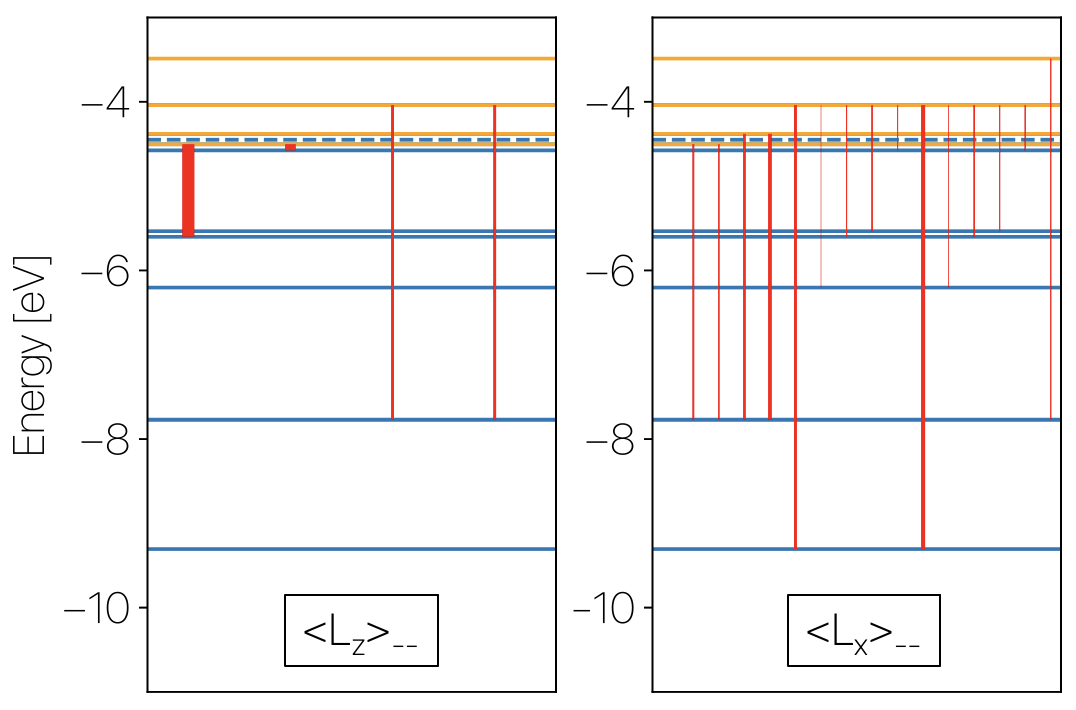
In this figure, the horizontal lines represent occupied (below the dashed line) MO while the lines above the dashed line are the unoccupied orbtials. Vertical lines represent non-vanishing $L$ components while the linewidth indicates the strength.

Subtle differences (i.e. lost of degeneracy) are caused by VASP’s periodic condition that breaks the rotational invariancce of the $d_{xy}$/$d_{x^2-y^2}$ orbitals.

The code used to generate these figures: 2023-01-12-MAE_decomposition.tar.gz.

Additional remarks:

• Within the rigid band approximation (the band structure as well as the orbital components of corresponding wavefunctions are fixed). We can adjust the Fermi level so that the occupations are changed. This way, since the MAE heavily depends on the coupling between occupied and un-occupied states, we can estimate how the MAE will change under sufficiently small doping. This is what Fig. 3(c) and 3(d) in PRL 110, 097202 (2013) show.

• For periodic systems, this method can be generalized by adding k-dependence, and we can have a plot of the MAE contribution of each k-point. The total MAE should be averaged using k-point weight.

• Up to now, we are treating $\lambda$ as a parameter (that, potentially, can be fitted if we know the true MAE value). However, in reaility, it needs to be calculated as $\braket{\phi\vert\lambda(r)\vert\phi}$ where $\phi$ is the radial part of the atomic wavefunctions, which also depend on the $l$ quantum numbers. In VASP, this is calculated within the PAW sphere using the all-electron partial waves (for details, see relativistic.F). If we really want to be percise, we can extract the exact values from VASP.