Pseudo-atom projected bandstructure with QE

Projected band structures are very useful tool that can help understanding the composition of the molecular orbitals. QE provides a program – projwfc.x to obtain projection coefficient (squared and abs’ed) so that projected band structure can be calculated.

However, the atomic wavefunctions it uses to project the Bloch waves onto are obtained from the pseudopotential files, which, can sometimes missing certain orbitals that one may want to project on. Also, for systems that has electrons localized at interstitial regions, one may need to project onto orbitals that are located at the off-atomic positions. One way to achieve this is to use a pseudo atom with everything set to $\sim 0$ except it’s pseudo atomic wavefunctions (PS-WFC).

As a demonstration, I’ve generated the pseudopotential of a pseudo hydrogen atom using the virtual_v2.x code. virtual_v2.x code allows generation of new PPs by combining PPs with different VCA weight. By default it can only blend two PPs together by setting the weight of one PP ($x$) and assuming the other to be ($1-x$). Here, however, we only need to scale down the PPs to $\sim 0$, while keeping the PS-WFC intact. I’ve modified the virtual_v2.f90 so that everything except the PS-WFC are scaled down to $0$. The modified source file for QE vertion 6.5 can be found: virtual_v2.f90.

After compiling, we can now generate a new a PP by assigning the weight of $0$ with the USPP H.pbe-rrkjus_psl.1.0.0.UPF. This artificially generated pseudo H’sPP file is attached here: H.UPF.

Now, we are ready to run some calculations!

Here, using LaRuSi as an example: LaRuSi_input.tar.gz

First, insert the hydrogen atom into the corresponding site, and set its PP to H.UPF in scf.in:

&CONTROL
  calculation='scf',
  outdir='./wfns',
  prefix='LaRuSi',
  pseudo_dir='.',
  verbosity='high',
  wf_collect=.TRUE.
/

&SYSTEM
  ibrav= 6,
  nat= 7,
  ntyp= 4,
  celldm(1)=8.050948,
  celldm(3)=1.682261,
  nbnd=80,
  ecutwfc=50,
  ecutrho=500,
!  tot_charge=-0.0001,
  input_dft='pbe',
  occupations='smearing',
  smearing='mp',
  degauss=0.005d0,
  nspin=1,
/
&ELECTRONS
  conv_thr = 1.0d-8
  electron_maxstep=300,
  mixing_beta = 0.7d0
/
&IONS
/
&CELL
  press_conv_thr=0.1
/
ATOMIC_SPECIES
  La 138.9055 La.pbe-spfn-kjpaw_psl.1.0.0.UPF
  Si 28.0855  Si.pbe-n-kjpaw_psl.1.0.0.UPF
  Ru 101.07   Ru.pbe-spn-kjpaw_psl.1.0.0.UPF
  H  1.0      H.UPF
ATOMIC_POSITIONS (crystal)
  Ru  0.0000000000  0.0000000000  0.0000000000
  Ru  0.5000000000  0.5000000000  0.0000000000
  Si  0.5000000000  0.0000000000  0.1665860000
  La  0.0000000000  0.5000000000  0.3156630000
  La  0.5000000000  0.0000000000  0.6843370000
  Si  0.0000000000  0.5000000000  0.8334140000
  H   0.5 0.5 0.5
K_POINTS {automatic}
  6 6 3 0 0 0

and run pw.x. Then, do an nscf calculation to get bands using band.in:

&CONTROL
  calculation='bands',
  outdir='./wfns',
  prefix='LaRuSi',
  pseudo_dir='.',
  verbosity='high',
  wf_collect=.TRUE.
/

&SYSTEM
  ibrav= 6,
  nat= 7,
  ntyp= 4,
  celldm(1)=8.050948,
  celldm(3)=1.682261,
  nbnd=80,
  ecutwfc=50,
  ecutrho=500,
!  tot_charge=-0.0001,
  input_dft='pbe',
  occupations='smearing',
  smearing='mp',
  degauss=0.005d0,
  nspin=1,
/
&ELECTRONS
  conv_thr = 1.0d-8
  electron_maxstep=300,
  mixing_beta = 0.7d0
/
&IONS
/
&CELL
  press_conv_thr=0.1
/
ATOMIC_SPECIES
  La 138.9055 La.pbe-spfn-kjpaw_psl.1.0.0.UPF
  Si 28.0855  Si.pbe-n-kjpaw_psl.1.0.0.UPF
  Ru 101.07   Ru.pbe-spn-kjpaw_psl.1.0.0.UPF
  H  1.0      H.UPF
ATOMIC_POSITIONS (crystal)
  Ru  0.0000000000  0.0000000000  0.0000000000
  Ru  0.5000000000  0.5000000000  0.0000000000
  Si  0.5000000000  0.0000000000  0.1665860000
  La  0.0000000000  0.5000000000  0.3156630000
  La  0.5000000000  0.0000000000  0.6843370000
  Si  0.0000000000  0.5000000000  0.8334140000
  H   0.5 0.5 0.5
K_POINTS (crystal_b)
8
0.000000 0.000000 0.000000 30
0.000000 0.500000 0.000000 30
0.500000 0.500000 0.000000 30
0.000000 0.000000 0.000000 30
0.000000 0.000000 0.500000 30
0.000000 0.500000 0.500000 30
0.500000 0.500000 0.500000 30
0.000000 0.000000 0.500000 30

Then, gather results and generate the band structure using bands.x with bandx.in:

&BANDS
  prefix="LaRuSi"
  outdir="./wfns"
  filband="band.dat"
/

Finally, run projwfc.x to get the projection coefficients proj.in:

&projwfc
   prefix = 'LaRuSi',
   outdir = './wfns',
   lsym = .FALSE.,
   filproj = 'LaRuSi-proj.dat'
/

Now, we have generated the two files needed for plotting:

band.dat.gnu
LaRuSi-proj.dat.projwfc_up

I’ve wrote a script to parse the LaRuSi-proj.dat.projwfc_up file into atomic contributions:

python parse.py band.dat.gnu LaRuSi-proj.dat.projwfc_up

A series of parsed data files will be generated, their naming convention is:

{atomic_number}-{atom_type}-{orbital_label}.dat

The projection coefficients of the hydrogenic orbital at the interstitail site can be found in the 7-H-1S.dat file.

To plot the band, use plot.py as:

python plot.py 7-H-1S.dat 13.2959

where the last number is the Fermi energy that can be found in scf.out

The result should look like: .

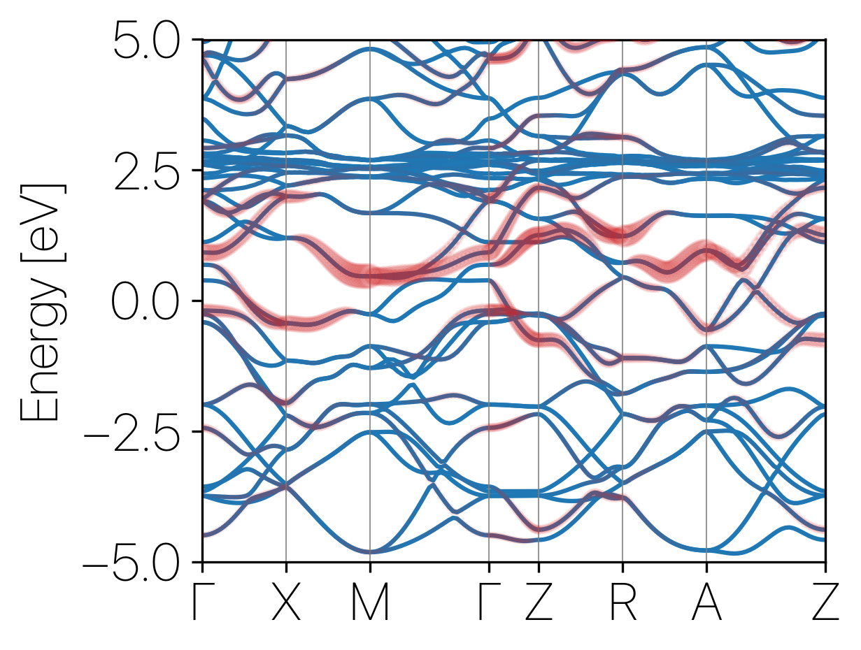NOTE: I’ve used 30 points between each high symmetry points, this is reflected in the plot.py file.

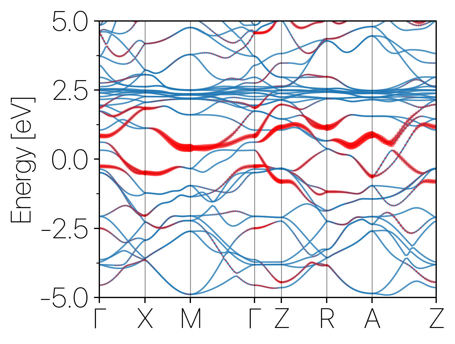
The same result can be obtained via VASP:

There are multiple ways of doing similar things with VASP, leave a comment down below and maybe I’ll post it later on😉.