Calculating spin texture from DFT and Wannier Hamiltonian.

Background

Spin texture describes the pattern which k-dependent spin directions formed in the Brillouin zone.

This peculiar phenomena arises from the coupling between spin and orbital motions of electrons – spin-orbital coupling (SOC). Without this coupling, the spin would remain in a “collinear” state and be rotationally invariant. However, when the SOC is introduced, spin moments are coupled to the anisotropic orbital degrees of freedom which makes them also anisotropic. This explains the origin of the magnetic anisotropy and the spin texture as well as other exotic phenomenas in condense matter physics. A rigorous derivation of the SOC Hamiltonian needs relativistic quantum mechanics with many-body interactions. However, here, I’m presenting a simple “pictorial” description of this phenomena: The orbital motion of electrons generates a magnetic field, and that magnetic field acts on the spin magnetic moment which makes it precess along that magnetic field direction (“Larmor” precession). This coupling will generate an energy splitting between different spin directions, hence changing the expectation value of the Pauli matrix.

A simple spin orbital Hamiltonian (can be added to the non-SOC Hamiltonian):

\textbf{H}_{soc} = \gamma \sigma \cdot L

where $S$ and $L$ are the spin operator(Pauli matrix) and the angular momentum operator, $\gamma$ is the spin-orbital coupling strength constant.

The Goal of this tutorial is to show you how to plot the spin texture directly from DFT and how to calculate it from diagonalising the Wanneir Hamiltonian and calculating the spin eigenvalues your self.

You may ask: If we can already get those directly from DFT then why do we need to do it again with Wannier functions? Well, I can only say it’s a fun thing to do. And it can be generalised if you want to, say, calculate the spin eigenvalues at specific K-point and Band number for an expended TB Wannier/TB Hamiltonian. (Which is an important thing for the topological people🤓)

In the following sections, I’ll use monolayer $\mathrm{In}_{2}\mathrm{Se}_3$ as an example to calculate spin texture. Note that because this is a 2D system, I’m plotting a 2D spin texture. For 3D systems, You can also plot them in 3D. Or you can still use 2D plot by slicing the Brillouin zone.

VASP

Implementation

VASP only consider the SOC effect in “the immediate vicinity of the nuclei” which they uses the PAW spheres as the boundary. This means they have to use the all-electron partial waves to calculate the spin orbital matrix element and subsequently the total add-on energy. If you take a close look at the source code, you will find the overlap is calculated by sandwiching the overlap operator:

\textbf{S} = \textbf{1}+\sum_{ij} Q_{ij} |\beta_{i}><\beta_{j}|

As long as we have the overlap operator, we can dot what ever we like to the Bloch functions!

How to?

VASP already provide the projected spin expectation value for each orbital (in x,y,z order) in the PROCAR file.

we can use pyprocar to plot it.

import pyprocar
pyprocar.repair('PROCAR') # usually needed.
pyprocar.fermi2D('PROCAR-repaired', outcar='OUTCAR', st=True, energy=-0.14, noarrow=False, spin=1, code='vasp')

Now, results!

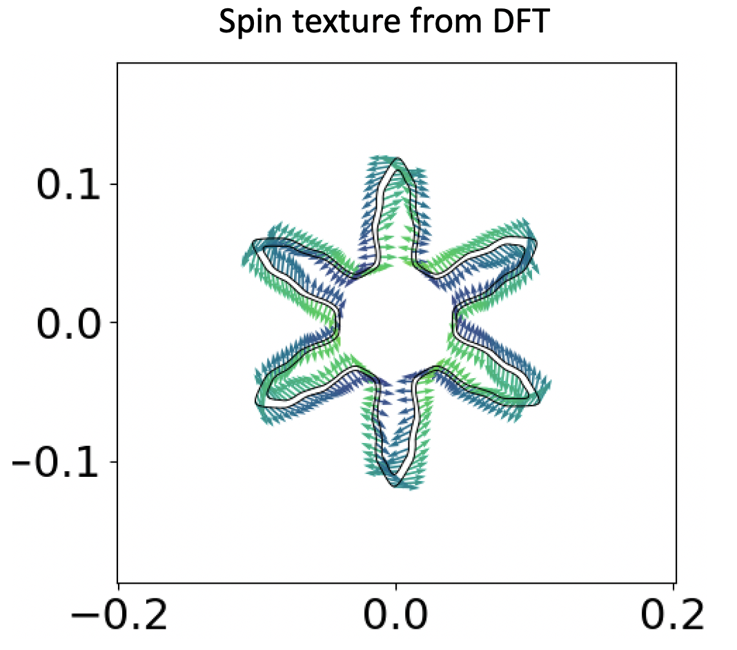
This is a 2D plot of the spin texture. The x and y axis are the rec. space vectors (well, not exactly. Since we have a hex cell, but you get the gist) and the arrows are the spin expectation vectors in the x-y plane, and the colour of those arrows correspond to the expectation values on the out of plane z direction. The cut energy is set to 0.14eV below the fermi level. As you can clearly see, we have 2 black circle-shaped thingy on the plot. They correspond to two different bands, and judging by the arrows, we can safely say they correspond to the opposite spin of a single orbital (in “collinear” sense, spin up and spin down).

Wannier90

Implementation

In the projection routine, VASP projects the Bloch functions onto a set of pure guiding functions with only one spinor component (this is not necessarily true, I’ve changed this behaviour in my fix, allowing one to specify spin quantisation axis, but I guess thats different). In the mean time, VASP doesn’t support writing spin matrix element for each k-point and band (yet, I’ll try to implement it in the future). So if the projection is skewed and we need to mix everything together by doing iterative minimisation (e.g. random projection and a large num_iter), then, we cannot guarantee the spinor components are well separated and our spin-textures are right. However, if our initial guess is pretty ‘on-the-spot’ (e.g. we can get perfect band interpolation without iterative minimisation). We are usually safe to assume that the end results are correct.

On a side note, I found that if the initial guess is good enough, even with some mixing, we can still get good results.

How to?

You need:

hr.dat file
.win file
\_band* file

If you don’t know how to calculate Wannier functions, click here!

I’ve decided to use pythtb as my diagonalisation tool (I’m lazy and I use python 2. Yeah, I know, I will port everything to python 3 tomorrow, I promise…)

Since the Hamiltonian and the Pauli matrix commute. After obtained the eigenvectors from diagonalising the Hamiltonian, we can apply the coefficients to the Pauli matrix and obtain the spin expectation value. As we are still in linear realm, we can sum up every orbitals’ coefficients (with the same spinor component) and apply the Pauli matrix to that big ‘all-in-one’ spinor wavefunction or apply Pauli matrix to each set of spinors for each orbital and added them up. Choose you warrior!

It’s coding time! (I use Atom and Hydrogen so #%% has special meaning, check it out!)

#!/usr/bin/env python

from pythtb import * # import TB model class
import matplotlib.pyplot as plt

# read output from Wannier90 that should be in folder named "example_a"
#   see instructions above for how to obtain the example output from
#   Wannier90 for testing purposes
InSe=w90(r"output/wannier90",r"wannier90")

# get tight-binding model without hopping terms above 0.01 eV
my_model=InSe.model()
#%% k_mesh parameters
ksize_x = 21
ksize_y = 21
krange = 1.0
origin = [-krange/2,-krange/2]

#%% set up k grid
k_vec = np.empty([(ksize_x)*(ksize_y),3])
for a in range(ksize_x):
    for b in range(ksize_y):
        k_vec[a*ksize_x+b]=[origin[0]+a*(krange/ksize_x),origin[1]+b*(krange/ksize_y),0.0]

# or use automatic generation (1st BZ, 1st quadrant only)
# k_vec = my_model.k_uniform_mesh([ksize_x,ksize_y,1])
(evals,evacs)=my_model.solve_all(k_vec,eig_vectors=True)

#%% reordering everything
# reorder kpoints
k_vec_new = k_vec.reshape(ksize_x,ksize_y,3)
# reorder evacs, need to swap axis to fortran like...
evacs_new = evacs.reshape(22,ksize_y,ksize_x,22).swapaxes(1,2)
# reorder evals, need to swap axis to fortran like...
evals_new = evals.reshape(22,ksize_x,ksize_y).swapaxes(1,2)

#%% get me spin expectatin value, see pauli matrix... duh.
nband = 16 # check band structure to see which band you want.... duh.
exp = np.empty([ksize_x,ksize_y,3],dtype=np.complex)
for a in range(ksize_x):
    for b in range(ksize_y):
        # for non-sprcified non-collinear spin channels, we use default order (orb1_up, orb1_down, orb2_up, orb2_down..)
        # this default order only works with Wannier90 v2.1.0+
        exp[a,b,0] = np.dot(np.conjugate(evacs_new[nband,a,b,0::2]),complex(+1,0)*evacs_new[nband,a,b,1::2])\
                   + np.dot(np.conjugate(evacs_new[nband,a,b,1::2]),complex(+1,0)*evacs_new[nband,a,b,0::2])
        exp[a,b,1] = np.dot(np.conjugate(evacs_new[nband,a,b,0::2]),complex(0,-1)*evacs_new[nband,a,b,1::2])\
                   + np.dot(np.conjugate(evacs_new[nband,a,b,1::2]),complex(0,+1)*evacs_new[nband,a,b,0::2])
        exp[a,b,2] = np.dot(np.conjugate(evacs_new[nband,a,b,0::2]),complex(+1,0)*evacs_new[nband,a,b,0::2])\
                   + np.dot(np.conjugate(evacs_new[nband,a,b,1::2]),complex(-1,0)*evacs_new[nband,a,b,1::2])

#%% plot spin texture
import matplotlib.transforms as mtransforms

fig, ax = plt.subplots()
# get tran_data function, this will slightly change the direction of the spin vector, but quantitavely its alrigh.
trans_data = mtransforms.Affine2D().skew_deg(-15, -15).rotate_deg(-15) + ax.transData

x = np.arange(origin[0],krange/2.,krange/ksize_x)
y = np.arange(origin[1],krange/2.,krange/ksize_y)

# M = exp[:,:,2].astype('float64') # use sigma_z as color map
M = evals_new[nband,:,:] # use eigenval as color map

im = ax.quiver(x,y,exp[:,:,0],exp[:,:,1],M, scale=13,pivot='mid',transform = trans_data)
# ax.axis([origin[0],krange/2,origin[1],krange/2])
ax.set_aspect('equal')
ax.set_title("band# "+str(nband))
plt.savefig("spintexture_band_"+str(nband)+".png", dpi=300)
# plt.show()

# %% plot fermi surface [or 3D band surface]
import matplotlib.transforms as mtransforms

fig, ax = plt.subplots()
im = ax.imshow(evals_new[17,:,:],
               extent=[origin[0],krange/2,origin[1],krange/2],
               aspect=1,interpolation='lanczos',origin='lower')
# skew and rotate to match k vectors.
trans_data = mtransforms.Affine2D().skew_deg(-15, -15).rotate_deg(-15) + ax.transData
im.set_transform(trans_data)
# reset axes limit
x1, x2, y1, y2 = im.get_extent()
ax.plot([x1, x2, x2, x1, x1], [y1, y1, y2, y2, y1], "-",
        transform=trans_data)

ax.set_title("band# "+str(nband))
plt.savefig("fermi_surface_band_"+str(nband)+".png", dpi=300)

Result time!

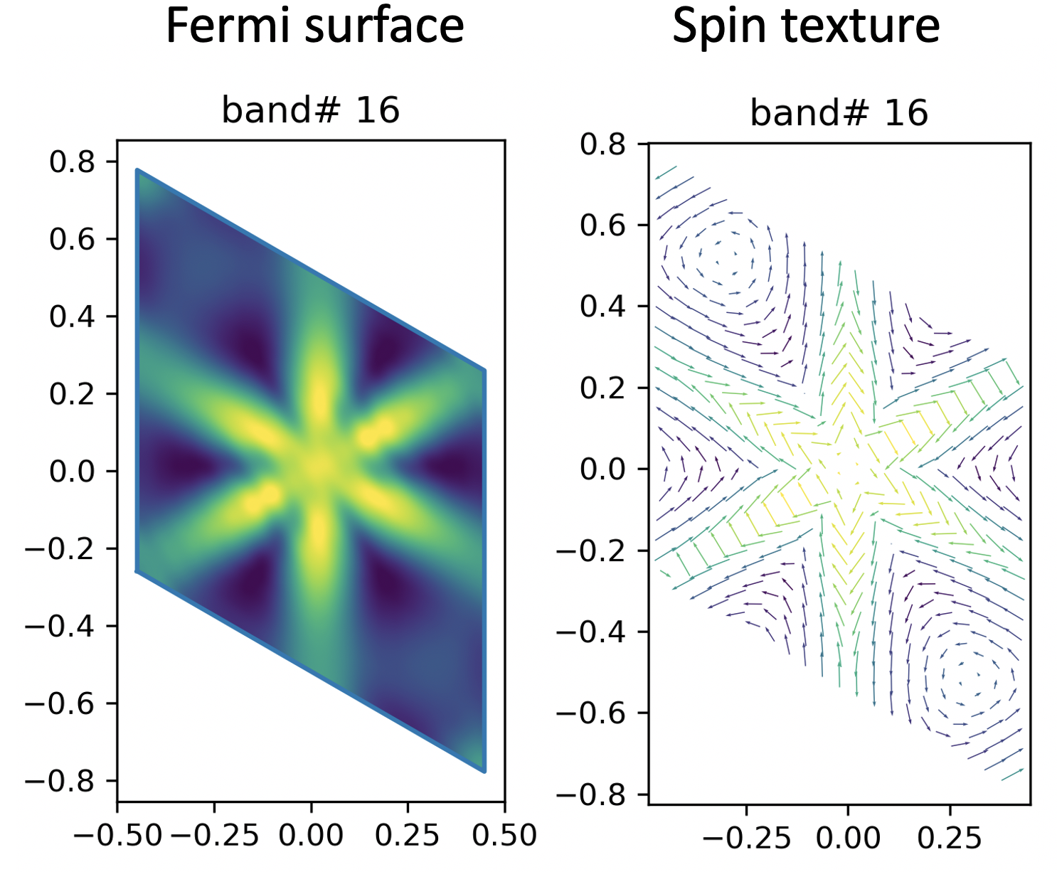
Here, I’m plotting the spin texture for two band (No. 16 and No. 17). I’m using the cut plane method here (contrary to the ‘direct from DFT’ method). Instead, I’m showing the eigenvalue of each band with different colour. Yellow -> higher in energy, Black -> lower in energy.

Well, to me, they look pretty good and similar to the DFT result.

Caveats

for Wanneir90 v2.1.0+, I’ve changed the default spinor order in the VASP2WANNIER90 interface. The new spinor orbital order (example):

site 1 projection s  (spin_1)
site 1 projection s  (spin_2)
site 1 projection px (spin_1)
site 1 projection px (spin_2)
site 1 projection py (spin_1)
site 1 projection py (spin_2)

the old spinor orbital order (example):

site 1 projection s  (spin_1)
site 1 projection px (spin_1)
site 1 projection py (spin_1)
...
site 1 projection s  (spin_2)
site 1 projection px (spin_2)
site 1 projection py (spin_2)

And you can always specify which component you want to project! Pretty neat huh?!

Input

I’ve put all input file in a zip file for download: VASP. Have fun computing!

2020-06-29 update

I’ve now implemented the .spn file output. The .spn file contains the spin matrix elements:

<\psi_{n,k} | \sigma_{x,y,z} | \psi_{m,k} >

By rotating this matrix with the U matrix we got from W90, we can calculate the spin expectation value @ each band and k point.

Again, since the Pauli matrix commutes with the Hamiltonian, they share a same set fo eigenvectors. We can use the eigenvectors from diagonalizing the Hamiltonian to get the same stuff.

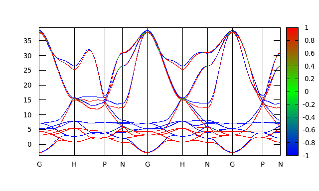
Here, just to confirm my implementation of .spn file is correct, I’ll compute the same spin projected bandstructure with Hamiltonian diagonalization and rotating the .spn file.

directly from rotating spn matrix

Just follow the Wannier90’s example17 and my example, you will get:

diagonalization method

For this to work, we need:

wannier90.win
wannier90_centres.xyz
wannier90_band.dat
wannier90_band.kpt
wannier90_hr.dat

Code to generate plottable file:

#!/usr/bin/env python

from pythtb import * # import TB model class
import matplotlib.pyplot as plt

Fe=w90(r"output/",r"wannier90")

# get tight-binding model without hopping terms above 0.01 eV
my_model=Fe.model()

#%%
# solve model on a path and plot it
path=[[0.0000, 0.0000, 0.0000],
      [0.500, -0.5000, -0.5000],
      [0.7500, 0.2500, -0.2500],
      [0.5000, 0.0000, -0.5000],
      [0.0, 0.0, 0.0],
      [0.500, 0.5000, 0.5000],
      [0.5, 0.0, 0.0],
      [0.0000, 0.0000, 0.0000],
      [0.75, 0.25, -0.25],
      [0.5, 0.0, 0.0]]
# labels of the nodes
k_label=(r'$\Gamma$',r'$H$', r'$P$', r'$N$', r'$\Gamma$',r'$H$', r'$N$', r'$\Gamma$',r'$P$')
# call function k_path to construct the actual path
(k_vec,k_dist,k_node)=my_model.k_path(path,500)

(evals,evacs)=my_model.solve_all(k_vec,eig_vectors=True)
# #%% get me spin expectatin value, see pauli matrix... duh.
exp = np.empty([18,500,3],dtype=np.complex)
for i in range(500):
    for b in range(18):
        exp[b,i,0] = np.dot(np.conjugate(evacs[b,i,0::2]),complex(+1,0)*evacs[b,i,1::2])\
                   + np.dot(np.conjugate(evacs[b,i,1::2]),complex(+1,0)*evacs[b,i,0::2])
        exp[b,i,1] = np.dot(np.conjugate(evacs[b,i,0::2]),complex(0,-1)*evacs[b,i,1::2])\
                   + np.dot(np.conjugate(evacs[b,i,1::2]),complex(0,+1)*evacs[b,i,0::2])
        exp[b,i,2] = np.dot(np.conjugate(evacs[b,i,0::2]),complex(+1,0)*evacs[b,i,0::2])\
                   + np.dot(np.conjugate(evacs[b,i,1::2]),complex(-1,0)*evacs[b,i,1::2])
#%% write everything to data
f= open("spinexp_band.dat","w+")
for i in range(18):
   for k in range(500):
        f.write('%s %s %s\n' % (k_dist[k], evals[i,k], np.real(exp[i,k,2])))
   f.write("\n")

f.close()

then plot with gnuplot:

set arrow from      0.34843,     -3.77527557 to       0.34843,     39.45894970 nohead
set arrow from      0.65018,     -3.77527557 to       0.65018,     39.45894970 nohead
set arrow from      0.8244,     -3.77527557 to       0.8244,     39.45894970 nohead
set arrow from      1.07078,     -3.77527557 to       1.07078,     39.45894970 nohead
set arrow from      1.41921,     -3.77527557 to       1.41921,     39.45894970 nohead
set arrow from      1.66559,     -3.77527557 to      1.66559,     39.45894970 nohead
set arrow from      1.91197,     -3.77527557 to      1.91197,     39.45894970 nohead
set arrow from      2.21372,     -3.77527557 to      2.21372,     39.45894970 nohead
unset key
set xrange [0: 2.38794]
set yrange [     -3.77527557 :     39.45894970]
 set xtics (" G "  0.00000," H "  0.34843," P "  0.65018," N "  0.8244," G "  1.07078," H
 "  1.41921," N " 1.66559," G " 1.91197," P " 2.21372," N "  2.38794)
 set palette defined (-1 "blue", 0 "green", 1 "red")
 set pm3d map
 set zrange [-1:1]
 splot "spinexp_band.dat" with dots palette

And we get:

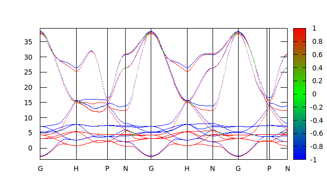
And again, this plot looks exactly like the one we obtained by directly rotating the spn matrix.

2021-07-04 update

I’ve finally updated the script to calculate spin expectation colored band using python3 (and now I’m using pybinding instead of pythtb) which gives me a huge speed bump.

To do the same thing as I did in 2020-06-29 update:

As a first step, we need to convert the Hamiltonian into a format that can be read by pybinding, using wanPB, we need:

wannier90_centres.xyz (add write_xyz=.true. to wannier90.win)
wannier90_tb.dat (add write_tb = .true. to wannier90.win)

simply use the following command in the same directory as the those two files resides in.

wanpb.x

Then, using the following script, we can generate the spinexp_band.dat data file:

import numpy as np
import pybinding as pb
pb.pltutils.use_style()
import matplotlib.pyplot as plt
import time
import sys


def progressbar(it, prefix="", size=60, file=sys.stdout):
    '''
    progress bar function from https://stackoverflow.com/a/34482761/12660859
    '''
    count = len(it)
    def show(j):
        x = int(size*j/count)
        file.write("%s[%s%s] %i/%i\r" % (prefix, "#"*x, "."*(size-x), j, count))
        file.flush()
    show(0)
    for i, item in enumerate(it):
        yield item
        show(i+1)
    file.write("\n")
    file.flush()

def get_node(kpts_scaled, rvec):
    '''
    convert scaled k points to absolute k points.
    '''
    kpts = []
    for kpt_scaled in kpts_scaled:
        kpts.append(kpt_scaled[0]*rvec[0]+
                    kpt_scaled[1]*rvec[1]+
                    kpt_scaled[2]*rvec[2])

    kpts = np.asarray(kpts)
    return kpts


def kpt_line_mode(kpts, nkpt=40):
    '''
    generate k paths using nodes
    '''
    segments = []
    segments_line = []
    node_line = []
    node_line_start = 0
    for seg in range(kpts.shape[0]-1):
        segment = np.linspace(kpts[seg],kpts[seg+1],nkpt)
        segments.append(segment)

        d_seg = np.linalg.norm(segment[1]-segment[0])
        node_line.append([node_line_start,node_line_start+d_seg*(nkpt-1)])
        node_line_start = node_line_start+d_seg*(nkpt-1)
        segments_line.append(np.linspace(node_line[seg][0],node_line[seg][1],nkpt))

    segments = np.concatenate(segments,0)
    segments_line = np.concatenate(segments_line,0)

    nkpt_tot = segments.shape[0]
    return segments, segments_line, node_line, nkpt_tot

# READ
#-----------------
# read-in lattice
lat = pb.load("wannier90.pbz")

# construct model
model = pb.Model(lat, pb.translational_symmetry())

# use lapack solver
solver = pb.solver.lapack(model)

# get me recripocal vectors
rvec = np.array(lat.reciprocal_vectors())

# INPUT
#-----------------
# construct high symmetry points.
#Gamma = [0,0,0]
#K1    = [0.5,-0.5,-0.5]
#M     = [0.7500, 0.2500, -0.2500]

path=[[0.0000, 0.0000, 0.0000],
      [0.5000,-0.5000,-0.5000],
      [0.7500, 0.2500,-0.2500],
      [0.5000, 0.0000,-0.5000],
      [0.0000, 0.0000, 0.0000],
      [0.5000, 0.5000, 0.5000],
      [0.5000, 0.0000, 0.0000],
      [0.0000, 0.0000, 0.0000],
      [0.7500, 0.2500,-0.2500],
      [0.5000, 0.0000, 0.0000]]


# RUN
#-----------------
# process k-points
#kpts_scaled = np.asarray([Gamma, K1, M])
kpts_scaled = np.asarray(path)
kpts = get_node(kpts_scaled,rvec)
segments, segments_line, node_line, nkpt_tot = kpt_line_mode(kpts, nkpt=40)

#%% diagonalize
bands=[]
eigvecs=[]
for kpoint in progressbar(segments, "K-points calculated: ", 20):
    solver.set_wave_vector(kpoint)
    bands.append(solver.eigenvalues)
    eigvecs.append(solver.eigenvectors)

#%% plot bands
nbnd = len(bands[0])
result = pb.results.Bands(segments_line, bands)
result.plot()

#%% convert to numpy array
evacs = np.asarray(eigvecs, dtype=complex)

#%% calculate spin expectation
exp = np.empty([nbnd,nkpt_tot,3],dtype=complex)

pauli = np.array([[[complex( 0, 0),complex( 1, 0)],[complex( 1, 0),complex( 0, 0)]],
                  [[complex( 0, 0),complex( 0,-1)],[complex( 0, 1),complex( 0, 0)]],
                  [[complex( 1, 0),complex( 0, 0)],[complex( 0, 0),complex(-1, 0)]]])

for i in range(nkpt_tot):
    for b in range(nbnd):
        evac = np.array([evacs[i,0::2,b],evacs[i,1::2,b]])

        exp[b,i,0] = np.dot(evac.conj()[0], np.dot(pauli[0], evac)[0])+np.dot(evac.conj()[1], np.dot(pauli[0], evac)[1])
        exp[b,i,1] = np.dot(evac.conj()[0], np.dot(pauli[1], evac)[0])+np.dot(evac.conj()[1], np.dot(pauli[1], evac)[1])
        exp[b,i,2] = np.dot(evac.conj()[0], np.dot(pauli[2], evac)[0])+np.dot(evac.conj()[1], np.dot(pauli[2], evac)[1])

#%% write to data
f= open("spinexp_band.dat","w+")
for i in range(nbnd):
   for k in range(nkpt_tot):
        # only write spin-z components to file (exp[i,k,2])
        f.write('%s %s %s\n' % (segments_line[k], bands[k][i], np.real(exp[i,k,2])))
   f.write("\n")

f.close()

Finally, using the same script, we can get the same spin expectation colored bandstructure.

NOTE-1: pybinding uses different notation as pythtb so the wavefunctions are bit different (with a phase), but that doesn’t affect our spin expectation calculations. However, if berryphase-like object is to be used, we need to be more careful with this.

NOTE-2: pythtb only read part (Rlatt>0 and some at the boundary) of the Wannier Hamiltonian whereas in parsing the wannier90_tb.dat file to pybinding, I simply used error handling to ignore all duplicates. This may incur some discrepencies between the two since the Wannier Hamiltonian may not be hermitian (which is weird). I need to doulbe check this.

NOTE-3: diagonalizing this Hamiltonian takes several minutes so I’ve added a progress bar. Simply decrease the k-mesh can significantly reduce the amunt of time needed to finish this plot.

NOTE-4: This script can be used as on general cases. Simply modify the K-nodes to whatever you want.